Richard Harris explores more of the mathematics of modelling problems with computers.
Last time I described the regular travelling salesman problem and we discovered that whilst the shortest tour was trivial to determine, the distribution of tour lengths was a little more difficult. Specifically, the factorial growth of the number of tours as the number of cities increased limited us to tours of no more than 14 cities.
So, how should we go about reducing the computational expense? Well, if we can spot any more symmetries we might be able to exploit them. Taking a look at every 5-city tour, fixing the first city as usual, might give a hint as to whether any more symmetries exist.
Figure 1 shows the complete set of tours for 5-city fixed-start regular TSP. Clearly there’s a symmetry we’ve not yet taken into account since only 4 of the 24 possible tours are distinct from one another!
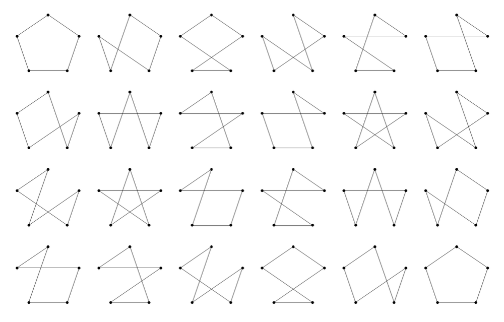 |
| Figure 1 |
So where is it?
Well, perhaps surprisingly, it’s the most obvious of them all. The fixed starting city and tour direction symmetries that we have already addressed exist for all TSPs. This final symmetry results from our tour being around a regular polygon. Specifically, it results from the fact that we can rotate and reflect the city labels on the polygon.
Trivially, reversing the city labels is equivalent to reversing the direction of the tour. More interestingly, rotating the city labels is not necessarily equivalent to rotating the starting city.
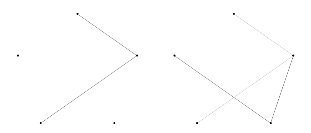
This is easily demonstrated by taking a tour that does not have rotational symmetry, say the second in Figure 1, rotating the labels and then checking whether rotating the starting point results in the same tour.
Figure 2 clearly shows that rotating the labels results in a tour that cannot be created by rotating the starting point.
| Rotating labels for a 5-city regular TSP | ||||||
|
||||||
| Figure 2 |
Before we embark on constructing an algorithm to efficiently generate the minimal set of symmetrically distinct tours, it’s probably worth figuring out how many of them there are. The analysis is easiest for tours with a prime number of cities, p.
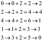
First of all, we should count the number of tours for which any rotation of the labels is equivalent to changing the starting city. Trivially, these tours must move the same number of vertices around the perimeter of the polygon at each step since if two consecutive steps were of different lengths, rotating the labels would mean that one of the cities would be followed by a different step, as illustrated in Figure 3.
 |
| Figure 3 |
For odd, and hence prime, regular tours there are

such tours (the factor of ½ resulting from the reflectional symmetry).
For prime regular TSPs, all remaining distinct tours must have a layout such that no rotation of the labels is equivalent to a rotation of the starting city.
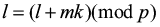
To see why, assume that rotating the labels k times, where k is not equal to either 1 or p, is equivalent to the initial tour with a different starting city. Rotating it another k times must also be equivalent, as must rotating it any multiple of k times, since we return to an equivalent of the starting tour every time. We should also note that rotating the labels more than p times is equivalent to rotating them that number modulo p.
For each label, l, and any multiple of the k rotations, m, l will be mapped to
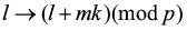
Now, it is a property of prime numbers that repeatedly applying this mapping must result in every number between 0 and p-1. For p equal to 5 and k equal to 2, we can demonstrate this by enumerating every step
Whilst this is a reasonable illustration of this fact, it is not remotely akin to a proof. To prove it, we first look for a multiple of the k rotations that maps every label to itself.
We can subtract the label value from both sides of the equation giving
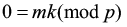
Since p is prime, mk can only be a multiple of p if either m or k is a multiple of p.
This demonstrates that if k is not equal to a multiple of p, repeatedly applying k rotations of the labels must generate all other rotations of the labels before returning to the initial layout. Therefore if k label rotations lead to a tour which is equivalent to the first, we simply keep repeating them to find that every possible rotation must also be equivalent.
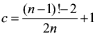
So the remaining distinct tours must generate 2p2, rather than 2p, tours since they have the extra rotational symmetry of the labels. The total number of tours must be equal to the sum of them both, giving
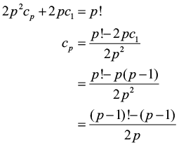
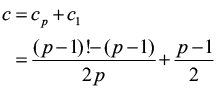
Hence the total number of distinct tours is given by
Whilst this does save us an extra order of magnitude, it’s still factorial complexity so it doesn’t really help us all that much.
For odd non-prime regular TSPs, the situation is even worse. This is because there will be some distinct tours for which there is a partial rotation of the labels that is equivalent to a rotation of the starting city. Since these will generate fewer tours, there must be more distinct tours.
For even regular TSPs, it is only the tour around the perimeter of the polygon for which label and starting city rotation are equivalent. This leads, by a similar argument, to a lower bound for the number of distinct tours being
The reason that this is only a lower bound is that, as for odd non-prime regular TSPs, there exist partial label rotations that are equivalent to starting city rotations which will each generate fewer tours.
I rather suspect that it’s not therefore worth the effort it would require to develop an efficient algorithm for enumerating the symmetrically distinct tours.
So how should we proceed?
Well, if we’re willing to sacrifice a little accuracy, we can simply generate a random subset of the tours. If the subset is large enough the resulting distribution of tour lengths should be approximately equal to that of the complete set of tours.
Fortunately for us, the standard library also includes a function for generating random permutations of sequences that we can use to generate our random tours; std::random_shuffle. Once again, we will ignore the reflectional symmetry for the sake of simplicity. We will still, however, exploit the rotational symmetry, although this time it’s to distribute the samples as evenly as possible amongst the full set of tours. Listing 1 shows sampling the tour histogram.
void
tsp::sample_tour(tour_histogram &histogram,
                 size_t samples)
{
  distances dists(histogram.vertices());
  tour t(histogram.vertices());
  generate_tour(t.begin(), t.end());
  while(samples--)
  {
    std::random_shuffle(t.begin()+1, t.end());
    histogram.add(tour_length(t, dists));
  }
}
|
| Listing 1 |
Since we’re no longer bound by the number of cities, but by the number of samples we might as well take a look at histograms for large numbers of cities.
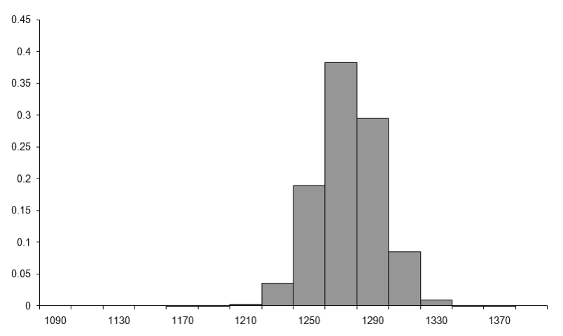
Figure 4 and Figure 5 record the results of 1,000 and 10,000 city regular TSPs, with 10,000,000 and 100,000,000 samples respectively.
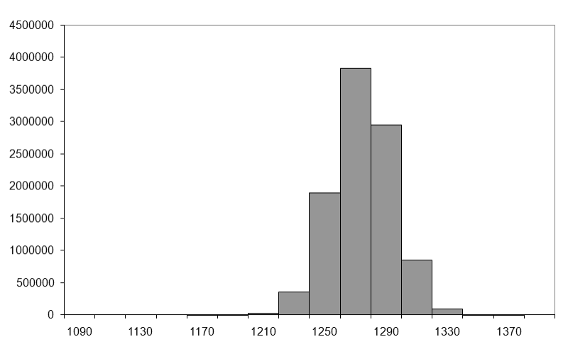 |
| Figure 4 |
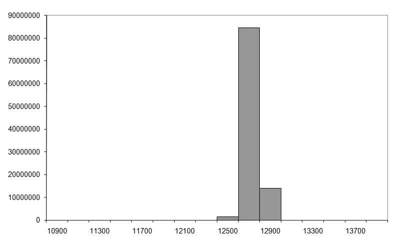 |
| Figure 5 |
Table 1 shows the approximate average tour lengths for these histograms.
|
|||||||||
| Table 1 |
It seems reasonable that the limit of the average tour length is going to be approximately 1.27n. The question that remains is why? Can we deduce a formula for the limit of the distribution of tour lengths for very large numbers of cities?
For extremely large numbers of cities, most steps in a regular TSP tour are more or less independent to those that have already been taken. It is only when the majority of cities have been visited that the choice of steps will be restricted to limited regions on the circumference of the polygon.
There is a statistical theorem called the law of large numbers which states that as n tends to infinity, the sum of n random numbers independently drawn from any single given distribution tends to n times the average of that distribution. If our assertion that the steps are more or less independent to each other is valid we should be able to approximate the average tour length with n times the average step length. For very large n, the average step length will be approximately equal to the average distance between two randomly selected points on the circumference of a circle of unit radius. In the same way that we can add up a finite set of step lengths and divide by the number of them to get the average, we can integrate the lengths of steps to cities separated by an angle of θ around the circumference and divide by 2π.
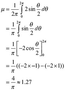
This clearly confirms that our expectation of the average tour length was correct, but is not enough for us to completely determine how the tour lengths are distributed.
There is another statistical theorem we can use to help us; the central limit theorem. The central limit theorem states, for a very wide class of distributions, that the sum of a set of independently drawn random numbers is normally distributed. Because of this property, it shows up in a vast number of places.
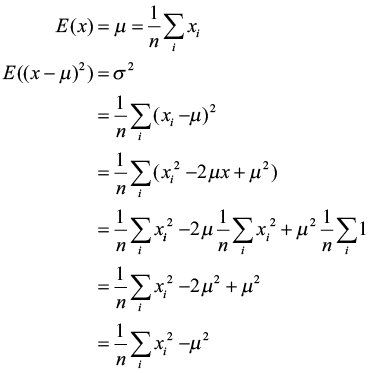
The normal distribution is defined in terms of both the average, μ, and the standard deviation, σ, of the numbers drawn from it. The standard deviation is a measure of how different on average the numbers in a set are from their mean and it is calculated as follows
Note that in this context E means the expected, or average, value.
Given these values the normal distribution is defined by its cumulative density function, or cdf, which is the function in x that gives the probability that a random number will be less than x.
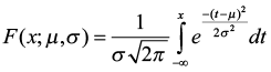
Unfortunately this integral does not have a closed form, meaning a simple formulaic, solution. The derivative, known as the probability density function, or pdf, is simple to calculate, however, and its graph is shown in Figure 6 (the normal distribution pdf).
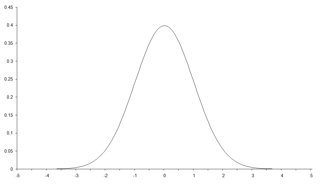 |
| Figure 6 |
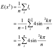
So the final piece of the puzzle is to calculate the average squared distance between two cities in a regular TSP, which we can use to determine which normal distribution is applicable. We could approximate it with an integral over the circle again, but there is an approximate formula for regular TSPs with a number of cities equal to a multiple of 4, so we may as well use it.
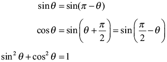
This may not look very easy to solve, but appearances can be deceptive. The trick is to exploit some trigonometric identities. It does get a little bit fiddly though, so those of you for whom the word ‘trigonometry’ conjures images of sinister maths teachers intent on ruining your life (or at least that double period after lunch on Thursdays) might want to skip ahead and just trust me.
Now, the identities in question are
We can use these by splitting the sum into four parts (Equation 1).
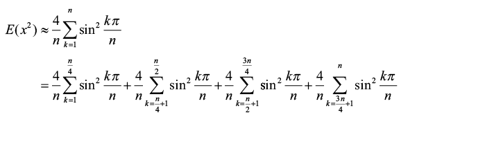 |
| Equation 1 |
Now since the last three terms are sums over ¼n steps offset by a constant factor, we can simply shift the constant factor from the index into the sum itself (Equation 2).
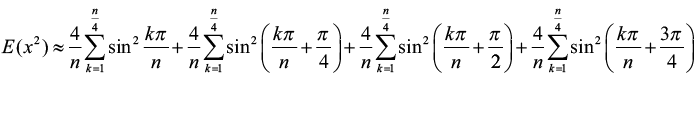 |
| Equation 2 |
The next point to note is that we can perform the second and fourth sums backwards by subtracting from the last angle in each sum (Equation 3).
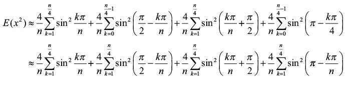 |
| Equation 3 |
Now we exploit the identity that equates the sine of the angle added to or subtracted from ½p to the cosine of the angle (Equation 4).
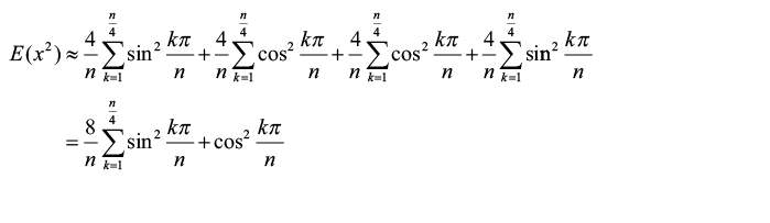 |
| Equation 4 |
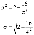
Finally, we exploit the identity that equates the sum of the squares of the sine and cosine of an angle to 1 to yield the result.
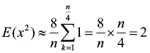
Therefore, the standard deviation of the step length is given by
In addition to stating that the sums of random numbers are normally distributed, the central limit theorem states that the specific normal distribution will have an average equal to n times that of their distribution and a standard deviation equal to the square root of n times that of their distribution.
This means that the distribution of tour length of a regular TSP with n cities should tend, for large n, towards
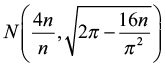
Figure 7 compares the histogram we’d expect from the normal distribution (at the bottom) to that we generated by sampling the 1,000 city tour (at the top).
 |
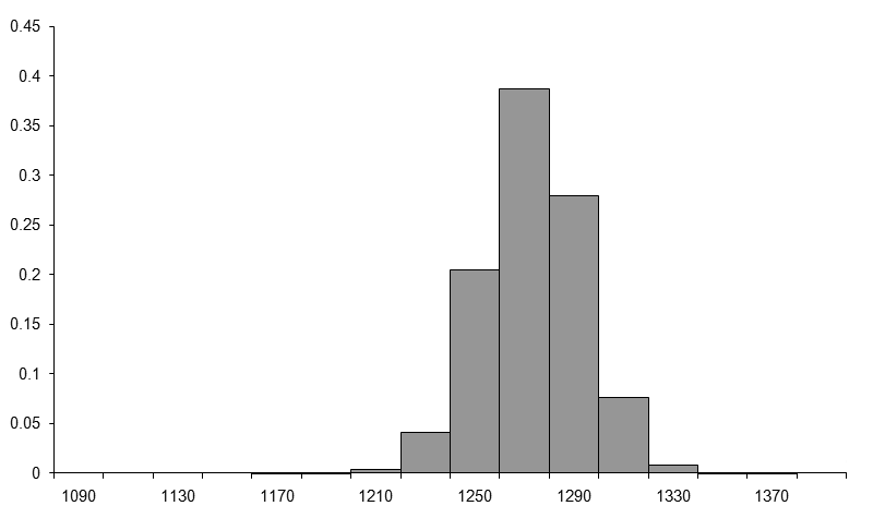 |
| Figure 7 |
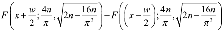
Under the assumption of normality, a bucket with mid point x and width w should contain the proportion of the samples given by
Well, despite the fact that the assumption that the tour steps are independent is demonstrably false these look remarkably similar, a fact borne out by the histogram of the difference between them, plotted on the same scale in Figure 8.
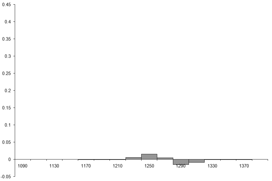 |
| Figure 8 |
In fact, there exists a mathematical technique for determining the likelihood that a sample histogram is consistent with a particular distribution. I strongly suspect that it would indicate that the sample histogram is not consistent with the normal distribution, but since we have already acknowledged that our assumptions are false we shouldn’t find that surprising. Nevertheless, given that the maximum difference is of the order of 0.015, or 1½%, it’s not too bad an approximation.
So can we perform a similar analysis on the usual type of TSP?
Well, let’s assume that the cities are evenly randomly distributed on the unit square. If we’re interested in the average tour length of all possible tours we should firstly note that we can take a tour of a random TSP by simply visiting each city in order. Furthermore, every possible tour can be generated by changing the labels and using the same scheme, since we can view the labels as instructions as to the order in which we should visit them. This means that picking the location of the next city in a TSP is equivalent to picking the next city in a tour. Since the former is independent of the cities already chosen, the latter must be independent the steps already taken, satisfying the independence requirement of the law of large numbers.
However, the distribution of step lengths is dependent on where in the square we are currently located, and this breaks the requirement that the step lengths are identically distributed. However, there is another version of the law of large numbers which states that the sum of independent random numbers from different distributions will tend to the sum of the averages of those distributions. Known as the strong law of large numbers, it requires that the standard deviations of those distributions have a particular property which happens to be satisfied if they do not grow without limit, or in other words are all less than some finite number. For cities in the unit square, this will be true for any reasonable definition of distance and so this approximation is actually more reasonable for normal TSPs than it is for regular TSPs.
Unfortunately, the expression for the average step length is a little bit more complicated this time. If we represent a pair of points by their coordinates on the unit square, (x, y) and (a, b), we have
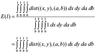
Once again, this is because the integral is the continuous limit of a sum. The fraction is the limit of the sum of the distances between all pairs of points in the unit square divided by the number of such pairs.
For the usual definition of distance, the integral becomes
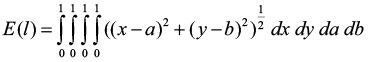
Whilst I’m not willing to assert that this does not have a closed form solution, it’s too complicated for me to attempt. If we change the cost of travelling between cities to the square of the distance, it becomes a little easier, however.
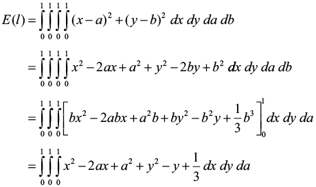
Continuing in the same vein leads to the result
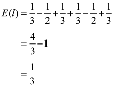
The average cost of a tour should therefore be approximately equal to ⅓n.
If you are interested, I invite you to investigate the accuracy of this approximation for different numbers of cities. You may be surprised as to just how accurate it actually is.
So is there anything more that can be said about the statistical properties of tours through TSPs? Well certainly, but not by me as I am afraid I have exhausted my mathematical toolbox. But this is an active area of research and a great many results have been found, of which just a few are described below.
Beardwood, Halton and Hammersley [Beardwood59] proved that the expected length of the shortest path through a random TSP tends to a value proportional to the square root of the number of cities.
Jaillet [Jaillet93] examined the probabilistic TSP in which each city has a probability that it may be skipped during the tour and provided bounds on the expected length of the shortest tour.
Agnihothri [Agnihothri98] examined the travelling repairman problem in which a repairman must travel to fix machines when they break down and developed a mathematical model with which expected travelling time, amongst other things, can be calculated.
And you, dear reader, may be able to shed further light on the properties of either the regular or normal TSP, and if you do please let me know.
Acknowledgements
With thanks to Larisa Khodarinova for a lively discussion on group theory that led to the correct count of distinct tours and to Astrid Osborn and John Paul Barjaktarevic for proofreading this article.
References
[Agnihothri98] Agnihothri, ‘A Mean Value Analysis of the Travelling Repairman Problem’, IEE Transactions, vol. 20, pp. 223-229, 1998.
[Beardwood59] Beardwood, Halton and Hammersley, ‘The Shortest Path Through Many Points’, Proceedings of the Cambridge Philosophical Society, vol. 55, pp. 299-327, 1959.
[Jaillet93] Jaillet, ‘Analysis of Probabalistic Combinatorial Optimization Problems in Euclidean Spaces’, Mathematics of Operations Research, vol. 18, pp. 51-71, 1993.
Further reading
Archimedes, On the Measurement of the Circle, c. 250-212BC.
Basel and Willemain, ‘Random Tours in the Travelling Salesman Problem: Analysis and Application’, Computational Optimization and Applications, vol. 20, pp. 211-217, 2001.
Clay Mathematics Institute ‘Millennium Problems’, http://www.claymath.org/millennium-problems.
Hoffman and Padberg, ‘Travelling Salesman Problem’, Encyclopedia of Operations Research and Management Science, Gass and Harris (Eds.), Kluwer Academic, Norwell, MA, 1996.
When he wrote this article, Richard had been a professional programmer since 1996. He had a background in Artificial Intelligence and numerical computing and was employed writing software for financial regulation.
We made a mistake…
In ‘The Model Student: The Regular Travelling Salesman – Part 1’ (Overload 171), we said that Archimedes proved that the ratio of the circumference of a circle to its diameter was between 31/7 and 310/71. He didn’t. He proved it was between 31/7 and 310/71.
Thank you to Gary Taverner for pointing out the error – but unfortunately we were too late to correct the printed version of Overload.
The error was spotted before the ePub version of Overload 171 was finalized, and has been corrected in the PDF and web versions.
Dr. Richard Harris died over the summer, and this article has been republished as a tribute to him, following on from the article in Overload 171.
For more information about Richard, his work and his legacy to the software industry, see ‘The Model Student: The Regular Travelling Salesman – Part 1’ in Overload 171.