The Duality…

Genetic algorithms can find solutions that other algorithms might miss. Anders Modén discusses their use in conjunction with back-propagation for finding better solutions.

Back then…

Many years ago, I was working on a numerical problem. I needed to solve an optimization problem in my work and I had a lot of trouble finding a good solution. I tried a lot of algorithms like the Gauss-Newton [ Wikipedia-1 ] equation solver for least-square problems and I tried the Levenberg-Marquardt algorithm (LM) [ Wikipedia-2 ] to improve the search for local optima.

All the time, my solution solver got stuck in some local optima. It was like being blind and walking in a rocky terrain, trying to find the lowest point just by touching the ground around you with a stick and guessing whether the terrain went up or down.

My intuition told me that the problem was related to the inability to look further away for low ground at the same time as looking for slopes nearby.

So I started to look for other solutions. I tried random searches and similar methods that use some sort of random trial, but in a problem with very large dimensionality, the random searches tried never found any ‘good’ random values.

I needed some kind of method that had a high probability of searching in places close to ‘old’ good solutions. If I found a local min going downwards I should continue to explore that solution. But at the same time, I needed to look far away in places I had never looked before at some random distance away. Not infinitely far away but at a normal distributed distance away. A normal distance has a mean value but can jump very far away [ Wikipedia-3 ].

Evolution

In my search for a suitable algorithm, I was eventually inspired by the evolution principles in Genetic Algorithms (GA) [ Wikipedia-4 ]. GA are a set of well-established methods used in the Genetic Evolution of Software and have been around since 1980. Initially used in simple tree-based combinations of logical operations, GA have the ability to define a large set of individual solutions. In this case, each solution is represented a local position in the rocky landscape with parameters in a non-linear polynomial equation. By building new solutions in new generations based on crossover and mutations, GA provided an iterative way both to explore local minima and to find new candidates further away. By setting up a normal distributed random function, I got a good balance between looking near and looking far away [ Springer19 ].

Cost function (or, how we reward our equation)

In order to solve a non-linear equation, we need to establish a criterion of how large an error a particular solution has. We usually identify this with different metrics like total least-squares using different norms. A simple least-square norm will do in this case [ Wikipedia-5 ]. By looking at the error (cost function) [ Wikipedia-6 ] in a large dimensional space, we get this rocky landscape. The LM method uses the gradient of this landscape to go along the slope to find a better solution. Furthermore, all the methods in back-propagation are also based on this stochastic gradient descent principle. Basically, it’s just a Newton-Raphson solver.

Solution

I wrote an algorithm to solve non-linear optimization problems using GA and I had a lot of fun just looking at the landscape of solutions where you could follow the progress of the algorithm. In the start there was just a large bunch of individual solutions randomly distributed in the numerical landscape.

In a while, some solutions were found that actually were better than the average and other solutions started to gather around these solutions. As the survival of the fittest kicked in, only the best solutions were saved. These clusters of solutions walked down the path to the lowest local point. At the same time, solutions started to be found further away. Sometimes they died out but sometimes they found new local optima. It was like following tribes of native inhabitants that settled, lived and died out.

Eventually the algorithm found better solutions than the LM algorithm. It wasn’t fast but it worked and solved my problem. When the job was done, I also forgot about it…

Almost present time

In 2013 I was impressed by the amazing results of AI and the start of deep learning. The technique behind convolution networks was so simple but very elegant. I felt I had to explore this domain and quite soon I recognized the behavior of the optimization problem. It was the same as my old non-linear optimization problems. I saw that the steepest gradient descent locally was just the same gradient descent as in LM and the rocky landscape was there. Lots of local minima, large plateaus of areas with little descent and the very large dimensionality of the solutions made my decision obvious. I needed to try to solve this by evolution…

I started to design a system that allowed me to try both traditional back-propagation as well as genetic evolution. I also wanted to build a system that allowed not only the optimization parameters to evolve but also the topology of the network. The structure of DNA inspired me as a key to both parameter values and to topology. By having an ordered set of tokens representing both parameters and connections, I could define an entire network by just using different tokens in a specific order.

The birth of Cortex API

I decided to build a software ecosystem both to verify my thoughts and to create a platform for experiments in genetic programming combined with neural networks. I named the software ecosystem Cortex, inspired by the neurons in our brain [ Modén16a ]. The requirements for the system were to be able to use both back-propagation and genetic evolution. I also wanted the system to allow any interconnectivity between neurons as our brain does and not only forward feed as most systems today do. The design should be based on DNA-like genetic elements.

Genetic element classes

In my design of Cortex, there are two classes of genetic elements (the smallest type of building block). The first class is the topology element. It defines the actual algorithm to be used in evaluation as a large connectivity graph. It is typically a chain of low level execution elements which we call the ‘topology DNA’. It is described as a fully generic network topology in high-level terms but can also be regarded as a sequence of DNA-based functions from input to output. These elements represent the connections between axons and dendrites in the human brain or in other animals.

The second element class is the activation or parameter class. It’s a set of variables that defines the activation and control of the first class network topology. It is also seen as a chain of ‘parameter DNA’, which is more or less the actual state of the brain. It represents the chemical levels that trigger the different synapses in the brain.

Toplogy DNA

The topology DNA is defined in my Cortex engine as a set of low-level instructions which all execute in a very defined sequence just like a stack-based state machine. The instructions are constructed so they can be randomly generated, communicate through registers and have local memory. The topology DNA is executed by a virtual machine just like a JVM, and a JIT compiler in the backend part can also accelerate it [ Modén18 ].

Parameter DNA

The parameter DNA is a set of register values used by the topology DNA for memory access and parameter control. Different algorithms in a population can have the same topology but individual parameter DNA. Maybe you can regard the topology DNA as the definition of the ‘creature’ and the parameter DNA is its personal skill or personality.

Genetic laws

The reproduction of a new generation of DNA is based on three basic genetic rules that affect parameter DNA

Crossover
Two parents’ DNA are combined in a number of ways. Some will be just new random outcomes but some will eventually inherit the good parts from both parents. Crossover can occur in one or multiple split points of the DNA chains. The dimensionality in a correctly constructed crossover is a subspace aligned with the gradients.
Mutation
A DNA position can be altered to a completely new DNA value. Typically created by chemical processes or radiation in real life. The dimensionality of this is high unless you limit the number of possible mutations in a DNA.
Biased crossover or breeding
This is a new term defined by the Cortex project but it is a very strong function. It uses two parents in a standard crossover but the results are biased towards a parent DNA value but not necessarily the same one. A crossover selects the same values from either parent. A breeding can be a linear combination with both positive and negative factors. An interpretation of the genetic law could be that it represents the ‘environmental’ effect (education, breeding or life experience) as you grow and it is not used in common GA as they are purely defined by genetic inheritance. This law allows a child to have genomes inherited as a function of parent’s genome. The dimensionality of this linear combination is still a subspace with a bounding volume aligned with the gradient as a convex hull which is extremely important.

There is also one genetic rule for topology DNA

Connectivity changes
The topology DNA is defined by instructions. The topology can be though of as an infinite number of neurons where all neurons are interconnected but with all weight factors set to zero. The Cortex Assembly Language simulates these neurons and their connectivity. By adding or removing instructions, you can simulate different topologies. Just like the other genetic laws, there are random additions of new routes between neurons. When the weights in the parameter topology are close to zero, the connections are removed.

These 4 rules are used to create new individuals in a new generation. The parameter DNA changes each new generation while the topology connectivity change seldom occur.

Simulation

A simulation is basically a loop running the genetic reproduction laws on a large number of successive generations. You start out with a start population that is a random set of individuals with random-generated DNA. The random values must have a normal distribution.

The number of individuals in the first generation represents the ‘survivor of the fittest’ and each new generation of new individuals will compete against this set. If their evaluated fitness function scores a value which is better that the worst fitness value in the first generation, the new individual will get into the ‘survivors set’ and the worst individual will die.

If the simulation is run in multiple instances on a distributed network, they all have different sets but the new candidates will be distributed if they manage to get in on the survivors list and then they will be able to get into other instances’ ‘survivor sets’. Eventually the sets will converge to a common set of individuals. Notice that this part doesn’t need any closed loop. Only the best DNA are broadcast and this is a huge benefit compared to back-propagation as you can scale this up without any limit.

Fitness function

In order to successfully rank the solutions in each generation, you need a global fitness function that can be evaluated for each individual. One cost isn’t enough as you are in this large multidimensional-parameter landscape. Instead you need a distribution of costs that can be compared. If your input/output contains a large set of input values and expected outputs and they follow the same statistical distribution, you can evaluate a statistical cost function using a large number of representative samples from a subset. The subset will follow the same distribution and can therefore be compared using different metrics like Frobenius norm, L2 norm or cost functions like SoftMax in back-propagation.

The Cortex engine combines the same cost functions used in back-propagation with the sampled cost function for the GA, which makes them use the same input/output and the same distribution of data.

Flow

In the beginning of a simulation, you may notice a high degree of chaos. Not that many individuals score really well, but after a while you will see a number of groups emerge. They represent a local max on the high-degree function surface. The mathematical solution is a very high-degree nonlinear function with multiple local min/max. In a traditional solver, you interpolate the gradients in the function to step towards the best local max value and this is seen as a successive improvement of the fittest in each local group generation by generation. BUT you will also eventually see new groups started far away from existing groups within completely new local min/max. A traditional LM solver will then not be able to find in its gradient search state, and many times this is also true for a deep neural network in its back-propagation when the problem is very flat with lots of local min/max, since this is a problem for the stochastic gradient search too.

This sudden emergence of a new group is really the strength of the evolution principle. A new ‘feature’ can be so dominant that new individuals now replace all offspring that were previously part of the ‘survivor’ groups. Some old strong genomes are often preserved for a number of generations but if they don’t lead to new strong individuals, they will be drained and disappear.

By having larger populations, the old strong genomes will survive longer and there is a higher probability that an old strong genome will combine with a future very new strong genome.

Building DNA

Let’s start with building a fixed topology network and select a very basic model.

To compare with other existing neural network APIs, we select a basic [input-4-4-output] network (see Figure 1).

" />

Figure 1

The code to realize this network in Cortex is shown in Listing 1.

// Create a brain
ctxCortexPtr cortex=new ctxCortex;

// define input output as derived classes of 
// my input and output
ctxCortexInput *input=new MyCortexInput();
ctxCortexOutput *output=new MyCortexOutput();

// Create an output layer that has the right size
// of output
output->addLayerNeurons(output->getResultSize());

// Add input/output to brain
cortex->addInput(input);

// Add input to brain
cortex->addOutput(output);

// create internal layers. two layers with 
// 4 neurons in each
cortex->addNeuronLayers(2,4);

// Connect all neurons feed forward
cortex->connectNeurons
  (CTX_NETWORK_TYPE_FEED_FORWARD);

Listing 1

The cortex layers are now defined and the connections (synapses) are connected using the forward feed pattern. All neurons between each layer are fully connected to each other.

Generating the code

We will now tell the network to generate an assembly a like program from the network that can be used to evaluate the network. First, we compile it…

  // Compile it and clear all internal data, 
  // possibly optimize it
  // cortex->compile(TRUE,optimize);

And then we set some random values in the DNA parameters…

  // Provide some random start values
  cortex->getContext()->
    randomParameters(1.0f/(neurons));

We now have generated an assembly-like program that in the future could possibly be run by a dedicated HW. We can take a look at the ‘disassembler’ of this program to understand the content.

The disassembly looks like Listing 2. The first section contains information about instructions and parameters. There are 33 value states. One for each node and one for each synapse. There is one input register and 33 parameter registers. These correlate to the node's different internal attributes. Compare with bias and weights in a normal network.

-- Compiled Cortex Program --
Instructions:311
ValueStates:33
Parameters:33
LatencyStates:0
SignalSources:1
InputSignals:1

------------ SubRoutines ---------------
 Threads:1
----------------------------------------

---- Thread:0 ----
 Offset:0
 Length:310
 Pass:0
 
---- Commands ----
RCL Input (0)       { Recall input register SP: +1 }
MULT Param (0)      { multiply with param register }
TEST Drop Value (0) { Test drop value register }
STO Value (0)       { Store value register SP: -1 }
RCL Value (0)       { Recall value register SP: +1 }
ADD Param (1)       { add param register }
NFU (7)             { Neuron function }
STO Value (1)       { Store value register SP: -1 }
RCL Value (1)       { Recall value register SP: +1 }
MULT Param (2)      { multiply with param register }
TEST Drop Value (2) { Test drop value register }
STO Value (2)       { Store value register SP: -1 }
RCL Value (2)       { Recall value register SP: +1 }
RCL Input (0)       { Recall input register SP: +1 }
MULT Param (3)      { multiply with param register }
TEST Drop Value (3) { Test drop value register }
STO Value (3)       { Store value register SP: -1 }
RCL Value (3)       { Recall value register SP: +1 }
ADD Param (4)       { add param register }
NFU (7)             { Neuron function }
STO Value (4)       { Store value register SP: -1 }
RCL Value (4)       { Recall value register SP: +1 }
MULT Param (5)      { multiply with param register }
TEST Drop Value (5) { Test drop value register }
.
. (CUT, see [Modén16b])
.
ADD Param (30)      { add param register }
NFU (7)             { Neuron function }
STO Value (30)      { Store value register SP: -1 }
RCL Value (30)      { Recall value register SP: +1 }
MULT Param (31)     { multiply with param register }
TEST Drop Value (31){ Test drop value register }
STO Value (31)      { Store value register SP: -1 }
CL Value (31)       { Recall value register SP: +1 }
SUM Stack (4)       { Sum stack values SP: -3 }
ADD Param (32)      { add param register }
NFU (7)             { Neuron function }
STO Value (32)      { Store value register SP: -1 }
RCL Value (32)      { Recall value register SP: +1 }
DROP                { drop stack value SP: -1 }
RCL Value (32)      { Recall value register SP: +1 }
DROP                { drop stack value SP: -1 }
----------------------------------------
 Passes:1
 MinLen:310
 MaxLen:310
 TotLen:310
 AvgLen:310
 Pass:0  Threads:1  Len:310  AvgLen:310

Listing 2

As you see above, the topology of synapses and neurons is translated into reading values from specific registers, doing some functions on the values and storing the value result in a new register.

Now this is an important statement. If we had an infinitely large network where all nodes were interconnected, we could model all networks just by the parameter values and set all weights to zero where we don’t have any synapses. This would result in an infinitely huge parameter DNA with just some sparse values and the rest being zeros. Instead, we divide the DNA into parameter DNA that has non-zero values most of the time and use a topology based on random interconnections modelled by the CAL instructions.

These two DNA parts are then kind-of exchangeable, where you can look at the parameters only or parameters and instructions together. This forms an important criterion in the evolving of the network. All mutations and crossovers and breeding are performed on the parameter DNA. During a simulation, the parameter DNA are evaluated and updated a lot. Then, every now and then, a network update occurs in an individual. A synapse is added with weight 0. This gives the same result as all the other cost-function evaluations but now we have a new parameter to play with. In the same fashion, a parameter that represents a weight that stays at zero for several generations could be exchanged for a removed synapse but in my simulations, I have chosen to let them stay so my network keeps growing but with more zeros.

Duality between GA and Neural Network Gradient Descent

As stated before, the strength of GA is in finding a new set of survivors far away from the current solutions. This is hard using a traditional LM but the LM is very good at incrementing the last steps to the best local solution; that is also true for the back-propagation method for Neural Networks using stochastic gradient descent. The GA takes a long time to find the ‘optimal local min/max’. It will find new solutions but they rely on random changes and not as targeted as the LM is.

So the duality exists between them. The GA will find new start points and the back-propagation of Neural Networks will find local min/max points. Cortex implements a hybrid mechanism that jumps between the two search modes.

Duality example

To exemplify the strength of the duality between Genetic Algorithms (GA) and Neural Network (NN) back-propagation a simple example is used [ Modén16c ].

In this example we use a simple target function like sin( x ). We want the neural network when given an input [0,2PI] to generate a sin( x ) curve. A sin( x ) curve is easy for us humans to recognize and we know that it can be described as a Taylor series of higher dimensions

The network knows nothing about the actual function but only the target value output for each x . We can choose any other function or non-continuous transfer function. It doesn’t matter. We are just interested in how a neuron network will simulate this and that it should be easy for us to look at it and understand it.

We start with a simple neural network with 20 neurons in each layer and just one mid layer. Listing 3 (overleaf) is the code to set up our start topology. We do no topology evolution in this example.

// Create a brain
ctxCortexPtr cortex=new ctxCortex;

// define input output as derived classes of 
// my input and output
ctxCortexInput *input=new MyCortexInput();
ctxCortexOutput *output=new MyCortexOutput();

// Create an output layer that has the right size
// of output
output->addLayerNeurons(output->getResultSize());

// Add input/output to brain
cortex->addInput(input);

// Add input to brain
cortex->addOutput(output);

// create internal layers. one layer with 
// 20 neurons in each
cortex->addNeuronLayers(1,20);

Listing 3

The input layer is a single neuron and the output is also a single neuron. We use the ELU (exponential linear unit) activation function and we train in batches of 10 samples in each batch. In total, we sample the sin function with 1000 steps, which gives us 100 iterations then for each epoch.

We initialize the neurons with zero mean and standard deviation of 1/20 (the number of neurons in each layer) and use a back-propagation step of 0.1. This is the result of the back-propagation…

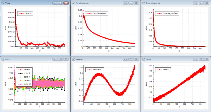
Let me explain the charts (see Figure 2)…

Figure 2

The most important chart is the ‘Error Magnitude’ chart (top right). It shows the error of the cost function for each iteration. This function should decrease as an indication of that we are learning. In this case we use a magnitude cost function L2 norm so it basically the sum of all squared errors in the estimated output function( x ) compared to sin( x ). When the cost function is zero, we have the correct output.

The next important chart is the ‘delta-err’ chart (bottom centre). It shows the error for each sample as a function of ( x ) compared to the sin( x ) target function. Optimally this will be zero for all values when the trained function is near or equal the target function sin( x ). As we define the function with 1000 values for x , we want the graph to show delta error = 0 for each x .

And the ‘value’ chart (bottom right) actually shows the estimated output function, which should be sin( x ) for each x . Right now we can see that the output is starting to get the shape of a straight line with some bends in the ends. As we just defined it using one layer, we have typically a network of parallel neurons that handles local segments of the transfer function.

The ‘delta’ chart (bottom left) shows the error propagated through the network for each iteration to the last node, which is the input node. Look at the delta values in back-propagation [ Wikipedia-7 ]. One delta for each connection but only the 5 first deltas are drawn. In a shallow network, it is quite easy to propagate delta to the last node so the magnitude are ‘rather’ high in this case. That means that the last layer is updated with ‘training’ information. If a network starts to learn, the deltas will increase.

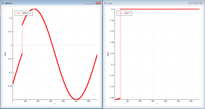
After a small number of iterations (20–100) we can see that the target function is looking like a sin( x ) curve. (See Figure 3.)

Figure 3

The delta error of the output is rippling around 0 but with pretty large values (1/100–1/10). We can draw the conclusion the network is learning. The cost error magnitude is continuously decreasing. As we have 20 neurons in parallel in the mid layer, we can continue to iterate to get better precision with smaller back-propagation steps. To make the neural network more sensitive to deep layers (making it less likely to get stuck in local optima), we just use a simple momentum as the gradient function. RMS or Adam would improve performance.

This first step shows that the back-propagation mechanism is very fast at finding solutions in the NN that converge to a sin function. This is done in seconds. The conclusion is that this feature is trained very easily in a shallow network using simple batch gradient descent.

But let’s see what happens in a deep network – or, at least, a deeper network – when we increase the layers and neurons. We now use 6 layers instead.

After a large number of iterations, the output is still just random (see Figure 4). The output doesn’t resemble the sin( x ) target function. The delta error shows that the output is pretty much a noisy dc level, which makes the error a noisy sin( x ). The deltas propagated through the network are now very low because each hidden layer kind-of reduces the energy in the back-propagation. The cost magnitude isn’t really decreasing and the system isn’t learning much at the beginning.

Figure 4

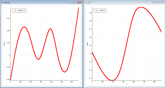
After a while, the training finally is able to kick some data through the network. Figure 5 shows the information after 14700 iterations.

Figure 5

The error magnitudes start to drop and the deltas propagated through the network start to increase. If we had selected a ReLU or a tanh activation function, it would have taken even longer to reach this state.

A deep network has a larger number of parameters and a larger ‘equation’ with many more minimums and saddle points, and therefore the gradient search mechanism – even if it is boosted with speed and momentum and other smart features – will take longer to iterate to a proper solution. Gradient selection methods like Adam and RMSProp are really good but they still struggle in deeper networks.

Now let’s introduce genetic training. In genetic training, the probabilities of finding solutions are not randomly equally distributed. There is a higher probability of finding solutions where the previous generations succeeded, which is the fundamental property of evolution. ‘The survival of the fittest’.

Figure 6 shows what genetic training can look like.

Figure 6

Genetic training uses evolution to find new candidates in the population. In the beginning, the first populations just contain garbage but very quickly (in this case in seconds) even if there are 6 layers and 20 neurons in each layer, the genetic algorithm finds a bit better candidate. The genetic algorithm doesn’t care about delta levels, so the innermost layers can instantaneously be updated by the genetic evolution.

The solutions found first have a value curve far from a sine and the delta-err is still a sine. But pretty quickly, the value curve starts showing sine-like shapes.

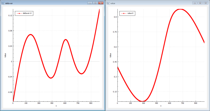
In this case (Figure 7) the genetic solver actually finds a better solution in a shorter time than the back-propagation mechanism.

Figure 7

The genetic solution will be a good one but perhaps not the very best we can find. It finds ‘global’ good solutions very quickly but the fine-grained tuned solutions will take a longer time to find (see Figure 8).

Figure 8

But the NN back-propagation, as noted before, was very efficient to iterate when a good solution was found. Can we use this to improve our genetic result?

We put the result from the genetic evolution into the NN back-propagation and we get Figure 9.

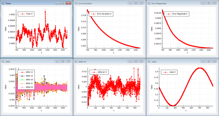
Figure 9

Instantly we can see that the NN back-propagation picks up a very good solution from the beginning. In this case we find a better solution than we previously found using only traditional back-propagation. The deltas are large from the start and the magnitude of error drops immediately. This shows that the solution found by the genetic evolution was a very good candidate and that the NN back-propagation is capable of iterating this solution to a better solution immediately.

This clearly shows the duality in one direction. The other direction is more trivial. You can feed better solutions into the GA using results from the NN and therefore improve the fittest solutions.

This result then defined the duality (state machine) between NN and GA.

I do believe the strong mechanisms of GA and the capability to run almost infinitely large parallel simulation either in the cloud or in Quantum Computers in the future will evolve the techniques of using GA.

Thanx for reading.

References

[Modén16a] Modén, A. (2016) CorTeX Genetic Engine, LinkedIn , 14 April 2016: https://www.linkedin.com/pulse/cortex-genetic-engine-anders-modén/

[Modén16b] Modén, A. (2016) CAL Execution Example, ToolTech Software , 1 June 2016: http://tooltech-software.com/CorTeX/execution_example.pdf

[Modén16c] Modén, A. (2016) Deep Genetic Training, ToolTech Software , 1 June 2016: www.tooltech-software.com/CorTeX/Deep_Genetic_Training.pdf

[Modén18] Modén, A. (2018) Cortex Assembler Language 2.0, LinkedIn , 10 July 2018: https://www.linkedin.com/pulse/cortex-assembler-language-20-anders-modén/

[Springer19] (2019) ‘Genetic Programming and Evolvable Machines’ on Springer Link: https://link.springer.com/journal/10710

[Wikipedia-1] Gauss-Newton algorithm: https://en.wikipedia.org/w/index.php?title=Gauss%E2%80%93Newton_algorithm&oldid=886266631

[Wikipedia-2] Levenberg-Marquardt algorithm: https://en.wikipedia.org/w/index.php?title=Levenberg%E2%80%93Marquardt_algorithm&oldid=888015378

[Wikipedia-3] Normal distribution: https://en.wikipedia.org/w/index.php?title=Normal_distribution&oldid=887884220

[Wikipedia-4] Genetic algorithm: https://en.wikipedia.org/w/index.php?title=Genetic_algorithm&oldid=887643125

[Wikipedia-5] Lp space: https://en.wikipedia.org/w/index.php?title=Lp_space&oldid=887448344

[Wikipedia-6] Artificial neural network: https://en.wikipedia.org/w/index.php?title=Artificial_neural_network&oldid=887630632

[Wikipedia-7] Backpropagation: https://en.wikipedia.org/w/index.php?title=Backpropagation&oldid=886645221

Anders Modén is a Swedish inventor working with software development at Saab Dynamics, which is a Swedish defence company building fighter aircraft and defence equipment. In his spare time he likes solving math problems and he plays jazz in a number of bands. He is also a 3D programmer and has written the Gizmo3D game engine (www.gizmosdk.se). He also develops the Cortex SDK in his private company, ToolTech Software.