What does complexity measurement mean? Roger Orr reminds us of the academic definition and looks at some real life situations.
Most computer programmers have heard of Order Notation – if you have studied computer science then it’s almost certain you’ll have studied this at some point during the course.
The notation is a way of describing how the number of operations performed by an algorithm varies by the size of the problem as the size increases.
But why do we care? Almost no-one is actually interested directly in this measure – but many people do care greatly about the performance of a function or algorithm. The complexity measure of an algorithm will affect the performance of a function implementing it, but it is by no means the only factor.
There are a number of different ways to measure the performance of a function, with overlap, or at least strong correlation, between many of them. Examples of common performance measures include:
- Wall clock time
- CPU clock cycles
- Memory use
- I/O usage (disk, network, etc)
- Power consumption
Complexity measurement is (normally) used to approximate the number of operations performed and this is then used as a proxy for CPU clock cycles and hence performance (or at least one of the measures of performance). However, it is a simplification of the overall algorithm; it may be a measure of only one of the operations involved and it may ignore other factors, such as memory access costs that have become increasingly important in recent years.
Introduction, or re-introduction, to order notation
Order Notation is a classification of algorithms by how they respond to changes in size.
It uses a big O (also called Landau’s symbol, after the number theoretician Edmund Landau who invented the notation). We write f ( x ) = O( g ( x )) to mean:
There exists a constant C and a value N such that
| f ( x )| < C | g ( x )| ∀ x > n
There may be a variety of possible ways of picking C and N . For example, consider the functions: f1 ( x ) = 2 x 2 + 3 x + 4 and f2 ( x ) = x 2 + 345678 x + 456789.
For f1 we notice that 3 x + 4 is less than x 2 when x is bigger than four. Hence f1 ( x ) < 3 x 2 , for x > 4. So we get C = 3, g ( x ) = x 2 and N = 4.
For f2 the numbers are a little larger but a similar method leads to seeing that f2 ( x ) < 2 x 2 for all values of x > 345678 and hence get C = 2, g ( x ) = x 2 and N = 345678; or we might start with a larger value for C , say 4000, and then have f2(x) < 4000 x 2 for all values of x > 87 hence get C = 4000, g ( x ) = x 2 and N = 87.
For the purposes of order notation it doesn’t matter what C and N are nor how large or small they are – they are constants; the important item is the function g () – in this example both f1 and f2 are the same complexity, O( x 2 ). In simple polynomial functions like these you don’t need to do the full analysis to find C and N as the complexity is simply the biggest power of x .
With more complex formulae it can be much harder to come up with appropriate constants and expressions; fortunately the complexity for many common algorithms is well-known (as we shall illustrate below).
Note too that for the O measure of complexity the function g may not be the smallest value needed. f3 ( x ) = 16 would usually be described as O(1) but can also be described as O( x 2 ) (with C = 1 and N = 4) but like any estimate it’s normally more useful the ‘closer’ it is and this function. This matters more for non-trivial algorithms where it may be very hard to exactly specify the best complexity function but much easier to specify a slightly larger one.
There are other symbols used in order notation such as the little-o symbol and the big-theta symbol. For example if both f ( x ) = O( g ( x )) and g ( x ) = O( f ( x )) then we can write f ( x ) = Θ( g ( x )). These are used in the mathematical theory of complexity but are generally less common in computer science.
Some common orders
Here a some common orders, with the slower growing functions first:
O(1) – constant
O(log( x )) – logarithmic
O( x ) – linear
O( x 2 ) – quadratic
O( x n ) – polynomial
O(e x ) – exponential
Order arithmetic
When two functions are combined the order of the resulting function can (usually) be inferred quite simply from the orders of the original functions. When adding functions, you simply take the biggest order.
eg. O(1) + O( n ) = O( n )
When multiplying functions, you multiply the orders
eg. O( n ) * O( n ) = O( n 2 )
So, more generally, when a function makes a sequence of function calls the overall order of the function is the same as the highest order of the called functions.
  void f(int n) {
    g(n); // O(n.log(n))
    h(n); // O(n)
  }
In this example f ( n ) = O( n .log( n )). This highest order is sometimes called the dominant complexity since as the number of items increases this value will dominate the overall complexity of the whole calculation.
For a function using a loop the order is the product of the order of the value of the loop count and the loop body
  void f(int n) {
    int count = g(n); // where the value of count
                      // is O(log(n))
    for (int i = 0; i != count; ++i) {
      h(n);           // O(n)
  }
Hence in this example too f ( n ) = O( n .log( n ))
Many standard algorithms have a well-understood order. One of the best known non-trivial examples is probably quicksort, which ‘everyone knows’ is O( n .log( n )). Except when it isn’t, of course! On average it is O( n .log( n )) but the worst-case complexity, for particularly unhelpful input values, is O( n 2 ).
Also, this is the computational cost, in terms of the number of comparison operations, not necessarily all operations or the memory cost.
The C++ standard mandates the complexity of many algorithms, using various different operation counts.
For example,
container
::size
:
Complexity: constant.
and
std::list::push_back
:
Complexity: Insertion of a single element into a list takes constant time and exactly one call to a constructor of T.
There are also various flavours of sorting. For example,
std::sort
:
Complexity: O(N log(N)) comparisons.
and
std::stable_sort
:
Complexity: It does at most N log 2 (N) comparisons; if enough extra memory is available, it is N log(N). (The standard is silent on what ‘enough’ means!)
and
std::list::sort
:
Complexity: Approximately N log(N) comparisons
The .Net documentation provides complexity for (some) algorithms. For example,
List<T>.Sort
:
On average, this method is an O( n log n ) operation, where n is Count; in the worst case it is an O( n 2 ) operation.
Java too provides complexity measures for some algorithms. For example,
Arrays.sort
:
This implementation is a stable, adaptive, iterative mergesort that requires far fewer than n lg( n ) comparisons when the input array is partially sorted, while offering the performance of a traditional mergesort when the input array is randomly ordered...
(The Java spec uses lg rather than log – but all logarithms have the same complexity so it is immaterial!)
However, unlike C++, neither .Net nor Java seem to provide much detail for the cost of other operations with containers. This makes it harder to reason about the performance impact of the choice of container and the methods used: not everything is dominated by the cost of sorting alone!
So that’s the theory; what happens when we try some of these out in an actual program on real hardware? Your own figures may vary because of machine and operating system differences (different clock speeds, varying amounts of memory, different speeds of memory access and cache sizes and different choices of memory allocation strategies).
strlen()
This seems like a straightforward function and at first sight measuring its complexity should be simple enough: O(
n
) where n is the number of bytes in the string. You may even have read some example source code for
strlen()
if and when you first learned C (see Listing 1).
int strlen(char *s) /* source: K&R */
{
  int n;

  for(n = 0; *s != '\0'; s++)
  {
    n++;
  }
  return n;
}
|
| Listing 1 |
Have you looked inside
strlen()
recently? Things have got much more complicated than this in practice! Here’s an extract from an implementation of the function on x64 – probably rather more than you wanted to know... (see Listing 2).
strlen:
    mov     rax,rcx       ; rax -> string
    neg     rcx
    test    rax,7          ; test if 64 bit aligned
    je      main_loop
    ; ...
    ; loop until aligned (or end of string found)
    ; ...
main_loop:
    mov     r8,7EFEFEFEFEFEFEFFh
    mov     r11,8101010101010100h
    mov     rdx,qword ptr [rax]      ; read 8 bytes
    mov     r9,r8
    add     rax,8
    add     r9,rdx
    not     rdx
    xor     rdx,r9
    and     rdx,r11
    je      main_loop
    mov     rdx,qword ptr [rax-8]
                    ; found zero byte in the loop
    test    dl,dl
    je      byte_0                  ; is it byte 0?
    test    dh,dh
    je      byte_1                  ; is it byte 1?
    shr     rdx,10h
    ; ... and the rest
byte_0:
    lea     rax,[rcx+rax-8]
    ret
|
| Listing 2 |
However, despite the re-write in assembly language and the tricks to enable checking 64 bits at once in the main loop this code is still O( n ).
Naïvely we write some code that calculates the elapsed time for a call to
strlen()
like this:
  timer.start();
  strlen(data1);
  timer.stop();
However, on most compilers in release mode the call appears to take no time at all ....
The reason for this is that calls to functions like
strlen()
can be optimised away completely if the return value is not used.
It’s vitally important with performance measuring to check you’re measuring what you think you’re measuring!
So we change the code to use the return value of
strlen()
and set up a couple of strings to test against:
  char const data1[] = "1";
  char const data2[] = "12345...67890...";
Compare time for
v1 = strlen(data1)
against
v2 = strlen(data2)
Once again, you may get a bit of a surprise, depending on which compiler and flags you’re using, as a call to
strlen()
of a constant string can be evaluated at
compile
time and hence is O(1) (also known as constant time.) I repeat – it’s vitally important to check you’re measuring what you
think
you're measuring!
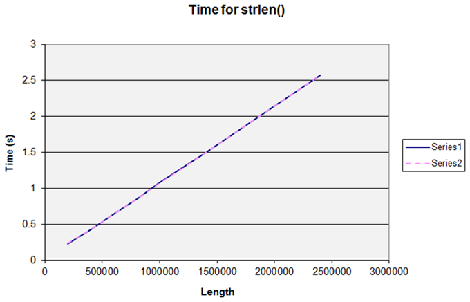
So for our third attempt we set up the string at runtime and now we get the graph we were expecting that demonstrates
strlen()
is O(
n
). (Figure 1.)
|
| Figure 1 |
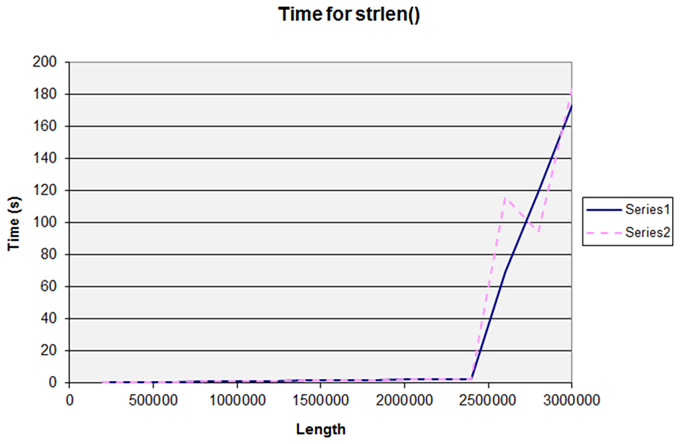
Series 1 and Series 2 are two separate runs over the same range of lengths, and demonstrate how repeatable the results are. However, this nice simple straight line graph breaks if we make the length a little larger. (Figure 2.)
|
| Figure 2 |
The graph is no longer linear and also no longer as consistent between runs. The reason is the the machine I used for this test has 2814Mb of RAM and the operating system starts swapping memory to disk as the size of the string gets near to this value.
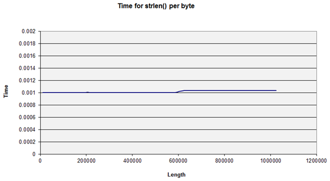
There is another anomaly with smaller strings too: this is present in the first graph above but not obvious to the naked eye. If we change the graph to display the average time for each byte we can see a jump at around 600,000 bytes. (See Figure 3.) Again, figures may differ on different hardware – this machine has 64K L1 + 512K L2 cache per core, ie. 589,524 bytes. So here we can see the effect of the cache size of this test.
|
| Figure 3 |
What we have demonstrated here is that the runtime execution time of
strlen()
is O(
n
) to a very good approximation when
n
is between cache size and available memory. The complexity in terms of the number of access operations on the string
is
still linear for larger strings than this but the effects of swapping dwarf this. It is likely that the cost of swapping is also O(
n
), but the ‘scaling’ factor
C
is much bigger (perhaps 250–300 times bigger in this case on this hardware).
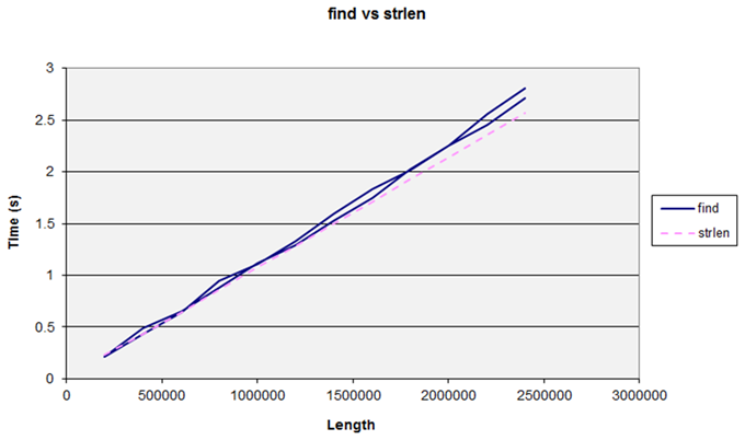
Let us see what happens if we try the same sort of operation but a slightly more generic algorithm by swapping over from using
strlen()
to using
string::find('\0')
We expect this will behave like
strlen()
and indeed it does – consistently slightly slower (Figure 4).
|
| Figure 4 |
Sorting
We now turn our attention to various sorting algorithms and how they behave under various conditions. We start with a (deterministic)
bogo
sort (see Listing 3).
template <typename T>
void bogo_sort(T begin, T end)
{
  do
  {
    std::next_permutation(begin, end);
  } while (!std::is_sorted(begin, end));
}
|
| Listing 3 |
This is not a sort you ever want to use in production code as it has O( n × n !) comparisons. Except when it doesn’t – here are some timings.
10,000 items: 1.13ms
20,000 items: 2.32ms
30,000 items: 3.55ms
40,000 items: 4.72ms
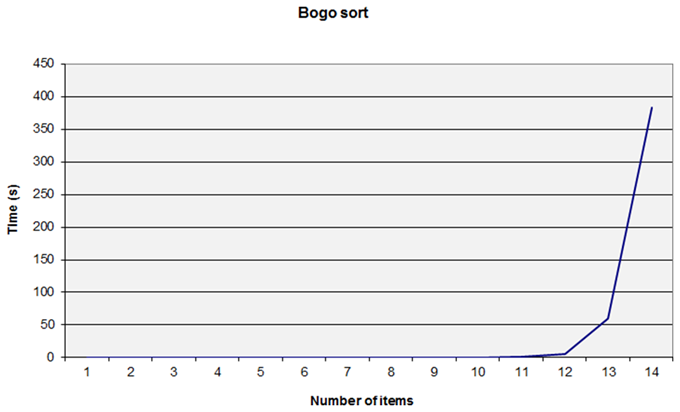
This appears to be O( n ) – but … how? I ‘cheated’ and set the initial state carefully. When measuring the performances of sorting you must be very careful about the best and worst cases. Make sure you are testing against similar data sets to those you will experience in real executions! In this case, I changed the generation of the data sets to use a randomised collection and then I obtained the expected sort of graph (Figure 5).
|
| Figure 5 |
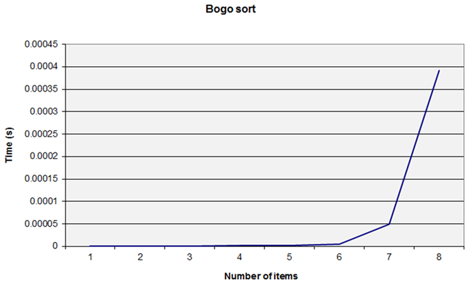
I didn’t do any runs with more than 14 items as the time taken was so long! You can see that we appear to hit a ‘wall’ at 13 or 14 items. But appearances can be deceptive – if we take the graph after eight items we get a similar ‘wall’ effect. (Figure 6.)
|
| Figure 6 |
While graphs can make some things easy to visualise they can also slightly mislead the eye: the wall effect seen here depends on the vertical scale of the graph.
What this means in practice is that the point at which the increasing complexity cost of a poor algorithm significantly affects the overall performance of the whole function or program will depend on what the relative timings are of the algorithm and the whole thing.
Let us leave the quaint bogo sort behind and try out some more performant flavours of sorting.
std::sort
which is the commonest used in C++,
qsort
the equivalent for C,
bubble_sort
which is easy to explain and demonstrate,
stable_sort
which retains the order of equivalent items and
partial_sort
which sorts the first
m
items from
n
(in this test I sorted the ‘top ten’ items).
(If you want to visualise some of these sort algorithms in practice I must mention AlgoRythmics – illustrating sort algorithms with Hungarian folk dance: https://www.youtube.com/watch?v=ywWBy6J5gz8 )
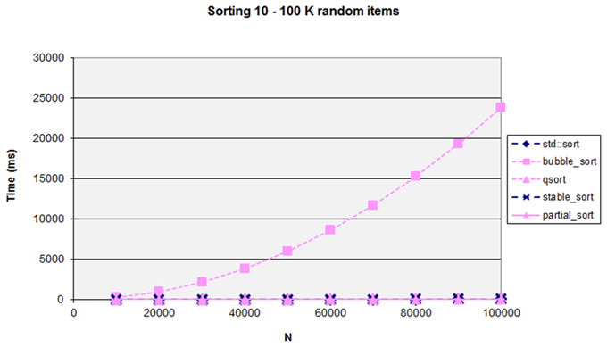
The dances do help to give some idea of how the algorithm works – they also show the importance of the multiplier C in the formula). (Figure 7).
|
| Figure 7 |
This graph might help to explain a quote from Andrei Alexandrescu: “ I’d like to go back in time and kill the inventor of bubblesort ”.
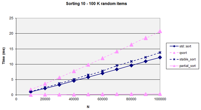
Removing this sort algorithm the graph now reveals the differences between the others (Figure 8).
|
| Figure 8 |
Notice that
std::sort
is faster than
qsort
which can come as a surprise to those who assume C is always faster than C++. It also shows that you do seem to pay a small cost for the stability of
stable_sort
. However, the real surprise for many people may be the excellent performance of
partial_sort
which is considerably faster than all of the other algorithms that sort the entire data set. When confronted with a sorting problem it is worth asking whether or not you need the
full
set sorted – if you only need a small number of the top (or bottom) items then
partial_sort
may prove to be a more performant solution.
However, that was with
randomised
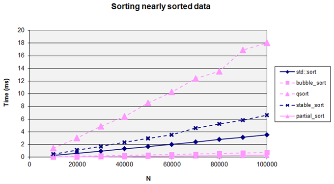
input data – in practice a lot of real data is not randomly sorted. When sorting
nearly
sorted data the
bubble_sort
algorthm can perform surprisingly well. (Figure 9.)
|
| Figure 9 |
This demonstrates how important it is to test performance in an environment as similar as possible to the expected target – many algorithms are sensitive to the input data set and if the test data set has different characteristics than the production data you may make a non-optimal choice.
Comparing and contrasting list and vector
The C++ collection classes, in common with some other languages, has a number of standard collection classes with slightly different interface and implementation. Two of these are
std::list<T>
and
std::vector<T>
. Both contain an ordered collection of values of type
T
, in the one case the underlying implementation is a doubly-linked list of nodes and in the other it is a contiguous array of objects. The C++ algorithm
std::sort
can be used to sort the vector, but not the list (since the list does not provide a random-access iterator). However, there is a member function sort in
std::list
. The complexity measure of
std::sort
is the same as
std::list::sort
– so what’s the difference in practice?
In terms of implementation, sorting a vector must actually copy the objects around inside the underlying array; whereas sorting a list can simply swap around the forward and back links without needing to move the payloads.
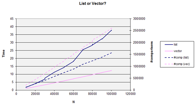
So let’s try it. Figure 10 plots two things at once: on the left hand axis we have the time to sort the collection and on the right hand axis the actual number of comparison operations performed (since the complexity is stated in terms of the number of comparisons).
|
| Figure 10 |
There are several points to note in this graph. Firstly, sorting the vector involves performing nearly twice as many comparisons as for the list when sorting the same data set, so while both are of the same theoretical complexity ( n .log( n )) the scaling of this ( C from the formula at the start of this article) is different. However, even though list does far fewer comparisons it is consistently slower than vector and gets more so as the number of items sorted increases.
This is a ‘worst case’ example as the object I used for this example merely wraps an integer, and so it is actually quicker to move the payload (1 machine word) than to swap the pointers in the list (2 machine words)!
The obvious question then is what happens as the size of the payload increases. If we retain the original payload as the ‘key’ comparison value then number of comparisons will remain exactly the same, the only change will be in the amount of data moved (for the vector). The list will continue to swap pointers and doesn’t even need to access the whole object.
I repeated the test above with gradually increasing sizes of payload for both vector and list. As expected, as the payload increased, the performance of the vector dropped until it eventually approximately equalled that of the list and then lagged behind it. However, I was surprised how large the payload size needed to be before this approximately equal performance was achieved: for this test on my hardware it was at around 100 bytes . I would have expected the increasing cost of copying to have had its effect more quickly.
One of the reasons is that, as we are all gradually coming to understand, modern computers perform very much better on data with good locality of reference. A vector is about as good as you can get in the regard – the objects in the vector are contiguous in memory and there are no additional control structures involved inside the data. While the specifics vary, the principle of locality is important and if it is multiplicative with the algorithmic complexity it can change the complexity measure of the overall function.
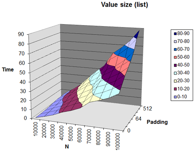
The performance of the list test is instructive in this regard: as discussed above when using the same value for the comparison the sort is doing exactly the same sequence of comparisons and link swaps. I found that sorting a list with a 1Kb payload took between two and three times as long as sorting a list of integers. At first I thought there might be a simple relation to the cache line size and that once the object payload exceeded the cache size (64b on my hardware) there would be no further effect on performance; but this did not seem to be the case. See below, the graph of time against the number of items sorted and the log of the object size. (Figure 11.)
|
| Figure 11 |
Perhaps we should be measuring the complexity of sort algorithms in other terms than just the number of comparisons?
Cost of inserting
Suppose we need to insert data into a collection and performance is an issue. Looking at the various standard containers we might be using, what might be the differences between using:
std::list
,
std::vector
,
std::deque
,
std::set
, or
std::multiset
?
To refresh your memory, the cost of inserting for each of these is:
-
std::list‘constant time insert and erase operations anywhere within the sequence’ -
std::vector‘linear in distance to end of vector’ -
std::deque‘linear in distance to nearer end’ -
std::setandstd::multiset‘logarithmic’
We are also affected by the time to find the insert point.
I tested randomly inserting 10,000 items into the various collections, with the following results:
-
std:list~600msvery slow – cost of finding the insertion point in the list
-
std::vector~37msMuch faster than list even though we’re copying each time we insert
-
std::deque~310msSurprisingly poor – spilling between buckets
-
std::set~2.6ms – our winner!
It can be significantly faster to use a helper collection if the target collection type desired is costly to create. In this example, if I use a
std::set
as the helper object and then construct a
std:list
on completion of the inserts then the overall time to create the sorted list drops to
~4ms
. The use of a helper collection will obviously increase the overall memory use of the program at the point of converting the source to the target collection, but the performance gains can be considerable.
If we change the insertion order from a random one to inserting 10,000 already sorted items, then the performance characteristics change again (there are two choices of sort order to select whether items are added to the front or to the back of the collection):
-
std:list~0.88msFast insertion (at known insert point)
-
std::vector~0.85ms (end) / 60ms (start)Much faster when appending
-
std::deque~3msRoughly equal cost at either end; a bit slower than a
vector -
std::set~2ms (betweenvectoranddeque)
This article is about order notation, so what happens to these numbers if we change the number of items? Let us try using ten times as many items:
-
std:list~600s (1000×) -
std::vector~3.7s (100×) -
std::deque~33s (100×) -
std::set~66ms (33×)
The cost of finding the insertion point for
std::list
dwarfs the insert cost. It is easy to overlook parts of an algorithm to discover later they have added significant hidden complexity.
Can we beat
std::set
?
C++11 has some additional associative collection classes that use hashing for improved performance (at the expense of removing the natural sort order). If we try a naïve use of
std::unordered_set
we find it is very slightly
slower
at 10K (~2.8ms vs ~2.6ms) but does out-perform
std::set
better at 100K items (~46ms vs ~66ms)
However, we may have additional knowledge about our value set and so can use a different hash function – as is the case in my test program where a trivial, and fast, identity hash function can be used. This enabled
std::unordered_set
to achieve times of ~2.3ms (10K) and ~38ms (100K).
Conclusion
The algorithm we choose is obviously important for the overall performance of the operation (measured as elapsed time). As data sizes increase we eventually hit the limits of the machine; the best algorithms are those that involve least swapping. For smaller data sizes the characteristics of the cache will have some effect on the performance.
While complexity measure is a good tool we must bear in mind:
- What are N (the relevant size) and C (the multiplier)?
- Have we identified the function with the dominant complexity?
- Can we re-define the problem to reduce the cost?
Making it faster
We’ve seen a few examples already of making things faster.
-
Compile-time evaluation of
strlen()turns O( n ) into O(1) - Can you pre-process (or cache) key values?
- Swapping setup cost or memory use for runtime cost
-
Don’t calculate what you don’t need (We saw that, if you only need the top
n
,
partial_sortis typically much faster than a full sort) -
If you know something about the characteristics of the data then a more specific algorithm might perform better – for example
strlen()vsfind(), sorting nearly sorted data, or a bespoke hash function.
Pick the best algorithm to work with memory hardware
- Prefer sequential access to memory over random access
- Smaller is better
- Splitting compute-intensive data items from the rest can help – at a slight cost in the complexity of the program logic and in memory use.
Acknowledgements
Many thanks to the Overload reviewers for their suggestions and corrections which have helped to improve this article.
Further reading
Ulrich Drepper ‘What Every Programmer Should Know About Memory’: http://people.redhat.com/drepper/cpumemory.pdf
Scott Meyers at ACCU ‘CPU caches’: http://www.aristeia.com/TalkNotes/ACCU2011_CPUCaches.pdf
Bjarne Stroustrup’s vector vs list test (especially slides 43–47): http://bulldozer00.com/2012/02/09/vectors-and-lists/
Herb Sutter’s experiments with containers: http://www.gotw.ca/gotw/054.htm and looking at memory use: http://www.gotw.ca/publications/mill14.htm
Baptiste Wicht’s list vs vector benchmarks: http://www.baptiste-wicht.com/2012/12/cpp-benchmark-vector-list-deque/