When your application is slow, you need a profiler. Paul Floyd shows us how callgrind and cachegrind can help.
The good news is that you’ve read my previous two articles on Valgrind’s memcheck tool, and now your application has no memory faults or leaks. The bad news is that your application is too slow and your customers are complaining. What can you do? There are plenty of options, like get faster hardware, better architecture/design of the application, parallelization and ‘code optimization’. Before you do anything like that, you should profile your application. You can use the cachegrind component of Valgrind to do this.
Let’s take a step back now for a very brief overview of profiling techniques. Profiling comes in several different flavours. It can be intrusive (as in you need to modify your code) or unintrusive (no modification needed). Intrusive profiling is usually the most efficient, if you know where to profile. The catch is that you usually don't know where to look. Profiling can use instrumented code, either instrumented at compile or link time or on the fly (which is the case for cachegrind and callgrind). Lastly, the profiler can be hardware based, for instance using the performance counters that are a part of Intel CPUs. as used by Intel Vtune. In addition to performing time based profiling, you can also perform memory profiling (for instance, using Valgrind’s massif), I/O profiling and so on.
Profiling should give a clear picture as to whether there are any significant bottlenecks in your code. If you see that one function is taking up 60% of the time, then it's a prime candidate for optimization. On the other hand, if you see that no function uses more than a few percent of the time, then you're probably going to need to look at higher level approaches than code optimization (or else you will have to optimize a lot of code to make a big difference).
In general, profiling tools will tell you the time spent in each function, inclusive and exclusive of time spent in calls to other functions. They may also tell you the time spent on each line of code. Callgrind and Cachegrind generate output that has a lot in common, like ‘time’ spent per function and line. The main differences are that Callgrind has more information about the callstack whilst cachegrind gives more information about cache hit rates. When you’re using these tools, you’re likely to want to use the GUI that is available to browse the results, KCachegrind. This is not part of Valgrind; as the name implies, it is part of KDE.
Cachegrind
Let’s start with a small example (see Listing 1). It’s deliberately bad, and as already noted above, a classic case for using a better algorithm.
#include <iostream>
#include <cmath>

bool isPrime(int x)
{
  int limit = std::sqrt(x);
  for (int i = 2; i <= limit; ++i)
  {
    if (x % i == 0)
    {
      return false;
    }
  }
  return true;
}

int main()
{
  int primeCount = 0;
  for (int i = 0; i < 1000000; ++i)
  {
    if (isPrime(i))
    {
      ++primeCount;
    }
  }
}
|
| Listing 1 |
Compiling and running this is easy, just use Valgrind with the
--tool=cachegrind
option.
$ g++ -g badprime.cpp -o badprime
$ valgrind --tool=cachegrind --log-file=cg.out
   ./badprime
I measured the time it took to run (in VirtualBox on a 2.8GHz Opteron that’s about 5 years old). Without cachegrind it took 1.3s. Under cachegrind that rose to 12.6s.
So what do we have. Well, I told Valgrind to send the output to cg.out . Let’s take a look at that (Figure 1).
==1842== Cachegrind, a cache and branch-prediction profiler ==1842== Copyright (C) 2002-2011, and GNU GPL'd, by Nicholas Nethercote et al. ==1842== Using Valgrind-3.7.0 and LibVEX; rerun with -h for copyright info ==1842== Command: ./badprime ==1842== Parent PID: 1758 ==1842== ==1842== ==1842== I refs: 922,466,825 ==1842== I1 misses: 1,234 ==1842== LLi misses: 1,183 ==1842== I1 miss rate: 0.00% ==1842== LLi miss rate: 0.00% ==1842== ==1842== D refs: 359,460,248 (349,345,693 rd + 10,114,555 wr) ==1842== D1 misses: 9,112 ( 7,557 rd + 1,555 wr) ==1842== LLd misses: 6,316 ( 5,119 rd + 1,197 wr) ==1842== D1 miss rate: 0.0% ( 0.0% + 0.0% ) ==1842== LLd miss rate: 0.0% ( 0.0% + 0.0% ) ==1842== ==1842== LL refs: 10,346 ( 8,791 rd + 1,555 wr) ==1842== LL misses: 7,499 ( 6,302 rd + 1,197 wr) ==1842== LL miss rate: 0.0% ( 0.0% + 0.0% ) |
| Figure 1 |
Some of this looks a bit familiar. There’s the usual copyright header and the column of
== <pid> ==
on the left. The part that is specific to cachegrind is the summary of overall performance, counting instruction reads (I refs), 1st level instruction cache misses (I1 misses), last level cache instruction misses (Lli), data reads (D refs), 1st level data cache misses (D1 misses), last level cache data misses (Lld misses) and finally a summary of the last level cache accesses. The information for the data activity is split into read and write parts (no writes for instructions, thankfully!). Why ‘last level’ and not ‘second level’? Valgrind uses a virtual machine, VEX, to execute the application that is being profiled. This is an abstraction of a real CPU, and it uses 2 levels of cache. If your physical CPU has 3 levels of cache, cachegrind will simulate the third level of cache with its second level.
There’s a further option that you can add to get a bit more information,
--branch-sim=yes
. If I add that option, then (in addition to adding another second to the run time) there are a couple more lines in the output (Figure 2).
==2345== ==2345== Branches: 139,777,324 (139,773,671 cond + 3,653 ind) ==2345== Mispredicts: 1,072,599 ( 1,072,250 cond + 349 ind) ==2345== Mispred rate: 0.7% ( 0.7% + 9.5% ) |
| Figure 2 |
That’s fairly straightforward, the number of branches, branches mispredicted (conditional and indirect branches). Examples of C or C++ code that produces indirect branch machine code are calls through pointers to functions and virtual function calls. Conditional branches are generated for
if
statements and the conditional ternary operator.
So far, nothing to get too excited about. In the directory where I ran cachegrind there is now a file
cachegrind.out.2345
(where 2345 was the PID when it was executing, as you can see in the branch prediction snippet above). You can control the name of the file that cachegrind generates by using the
–cachegrind-out-file
option. Here’s a small extract. It’s not meant for human consumption (Figure 3).
desc: I1 cache: 65536 B, 64 B, 2-way associative desc: D1 cache: 65536 B, 64 B, 2-way associative desc: LL cache: 1048576 B, 64 B, 16-way associative cmd: ./badprime events: Ir I1mr ILmr Dr D1mr DLmr Dw D1mw DLmw Bc Bcm Bi Bim fl=/build/buildd/eglibc-2.15/csu/../sysdeps/generic/dl-hash.h fn=_init 44 1 0 0 0 0 0 0 0 0 0 0 0 0 45 1 0 0 0 0 0 0 0 0 0 0 0 0 46 13 0 0 4 1 0 0 0 0 4 3 0 0 49 16 0 0 0 0 0 0 0 0 0 0 0 0 50 8 0 0 0 0 0 0 0 0 0 0 0 0 63 8 0 0 0 0 0 0 0 0 0 0 0 0 68 1 0 0 0 0 0 0 0 0 0 0 0 0 |
| Figure 3 |
You can make this slightly more digestible by using
cg_annotate
. You just need to enter
cg_annotate cachegrind.out.<pid>
and the output will go to the terminal. Figure 4 is what I got for this example.
--------------------------------------------------------------------------------
I1 cache:         65536 B, 64 B, 2-way associative
D1 cache:         65536 B, 64 B, 2-way associative
LL cache:         1048576 B, 64 B, 16-way associative
Command:          ./badprime
Data file:        cachegrind.out.2345
Events recorded:  Ir I1mr ILmr Dr D1mr DLmr Dw D1mw DLmw Bc Bcm Bi Bim
Events shown:     Ir I1mr ILmr Dr D1mr DLmr Dw D1mw DLmw Bc Bcm Bi Bim
Event sort order: Ir I1mr ILmr Dr D1mr DLmr Dw D1mw DLmw Bc Bcm Bi Bim
Thresholds:       0.1 100 100 100 100 100 100 100 100 100 100 100 100
Include dirs:
User annotated:
Auto-annotation:  off

--------------------------------------------------------------------------------
         Ir  I1mr  ILmr          Dr  D1mr  DLmr         Dw  D1mw  DLmw          Bc       Bcm    Bi Bim
------------------------------------------------------------------------
922,466,826 1,234 1,183 349,345,693 7,557 5,119 10,114,555 1,555 1,197 139,773,671 1,072,250 3,653 349  PROGRAM TOTALS

--------------------------------------------------------------------------------
         Ir I1mr ILmr          Dr  D1mr  DLmr        Dw  D1mw DLmw          Bc     Bcm    Bi Bim  file:function
--------------------------------------------------------------------------------
895,017,739    1    0 340,937,515     0     0 5,000,000     0    0 135,559,306 968,532     0   0  badprime.cpp:isPrime(int)
 16,000,000    0    0   5,000,000     0     0 4,000,000     0    0   2,000,000       8     0   0  std::sqrt<int>(int)
 10,078,513    2    1   3,078,503     0     0 1,000,003     0    0   2,000,001  94,081     0   0  badprime.cpp:main
|
| Figure 4 |
Still it isn’t very easy to read. You can see the same sort of notation as we saw for the overall summary (I – instruction, D – data and B – branch). I’ve cut the full paths to the file:function part. You can filter and sort the output with the
–threshold
and
–sort
options. You can also generate annotated source either with
-auto=yes
or on a file by file basis by passing the (fully qualified) filename as an argument to
cg_annotate
. I won’t show an example here as it is rather long. Basically it shows the same information as in the
cg_annotate
output, but on a line by line basis. Lastly for
cg_annotate
, if you are using it for code coverage metrics, then you can combine multiple runs using
cg_merge
.
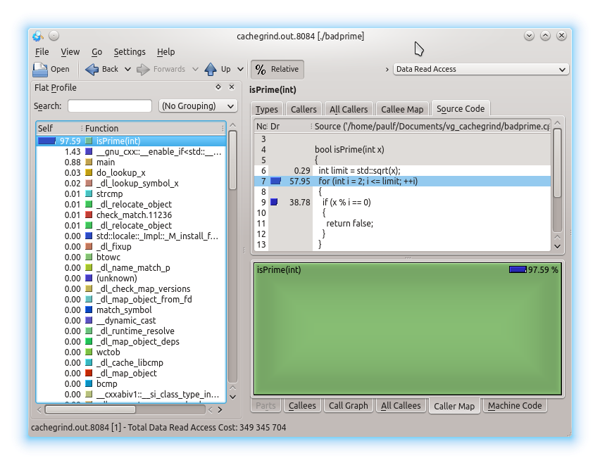
As already mentioned, you can use Kcachegrind. This is a fairly standard GUI application for browsing the performance results. It isn’t part of Valgrind, rather it is a component of KDE so you may need to install it separately. If you want to be able to see the funky graphics, you’ll need to have GraphViz installed. Figure 5 is a screen shot showing, on the left, percent of total time per function in descending order. The top 3, as expected, are the awful
isPrime
,
sqrt
and
main
with 99.9% between them. On the top right I’ve selected the Source Code tab, and we can see three lines with percent of time next to them. In this small example, the other tabs aren’t very interesting.
|
| Figure 5 |
Most of the navigating can be done by clicking the list of functions in the left pane. You can search for functions and also filter by the following groups – none, ELF object, source file, C++ class and function cycle. The two right panes have similar displays, roughly for displaying information about callers and callees (that is, functions called by the current function). Clicking on the % Relative toggle switches between showing absolute units (e.g., instruction fetches) and the percentage of the total. The drop down box on the top right allows you to display cache hit/miss rates, instruction fetches and cycle estimates.
Callgrind
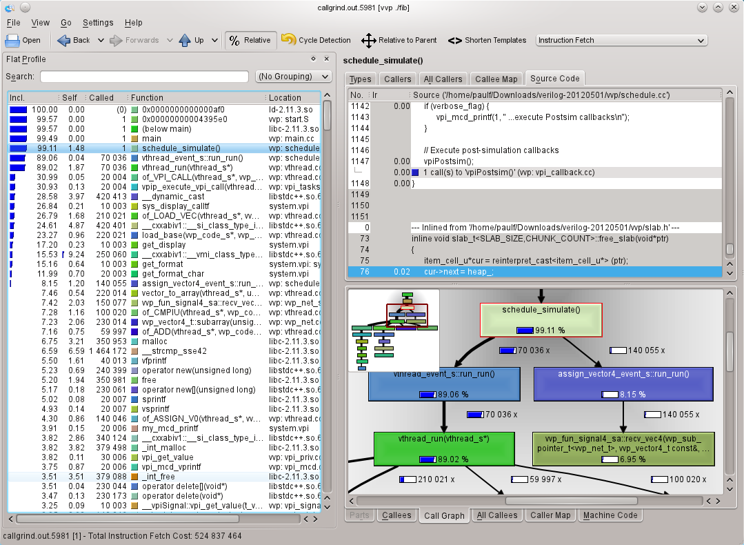
For an example using callgrind, I downloaded and built a debug version of Icarus Verilog [ Icarus ] and compiled and simulated a Fibonacci calculator [ Fibonacci ] with small modifications to make the simulation last longer and exit on completion).
The commands that I used were:
iverilog -o fib fib*.v
for the compilation, and
  valgrind --tool=callgrind
  --log-file=callgrind.log vvp ./fib
to profile the simulation.
Finally
kcachegrind callgrind.out.5981
to view the results (see Figure 6).
|
| Figure 6 |
This time, there isn’t all of the cache hit/miss rate information, but instead there is far more on the interrelations between functions and time. You can navigate through the functions by double clicking in the call graph.
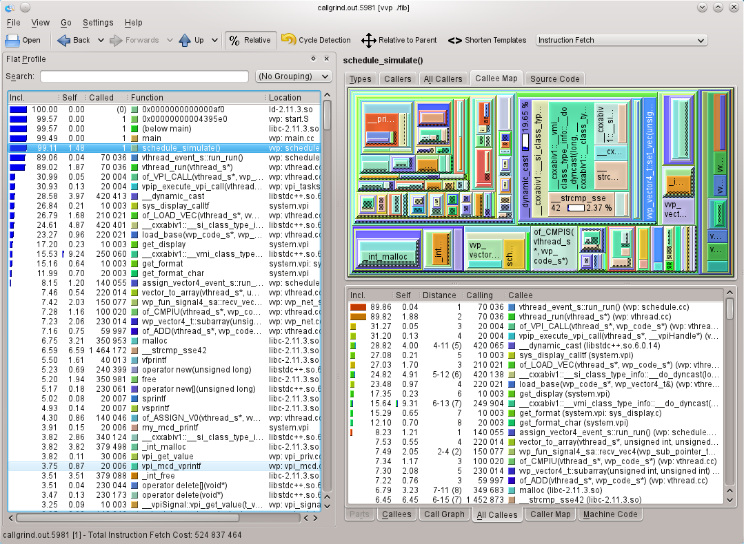
In the last snapshot, I show the funky callee map (which I expect will look better in the PDF version of the magazine in colour than in the black and white print magazine). The areas of the rectangles is proportional to the time spent in the function. Very pretty, but when it’s as cluttered as this example, it’s not much use. Both the map and the list are dynamic, and you can click in one and the area or list item will be highlighted in the other. You can also double click to jump to a different function. When you are navigating like this, you can use the back/forwards buttons on the toolbar to navigate in a similar fashion to a web browser, or navigate up the call stack (see Figure 7).
|
| Figure 7 |
Callgrind has
callgrind_annotate
that is a text processor for its output files. This is the callgrind equivalent of
cg_annotate
, and since the output is very similar, I won’t show it here.
Practical difficulties
One problem that I’ve experienced with callgrind was with differences between the floating point results with and without callgrind. In this case, I encountered numerical instability with callgrind that I didn’t get when running the application natively. This is worse for 32bit x86, where by default code gets generated to use the venerable x87 floating point coprocessor. This uses 10byte (80bit) precision internally. Usually this means that if you have an expression that involves several operations on doubles, the operations will be done at 80bit precision and the result converted back to double precision (8byte, 64bit, required by the C and C++ standards). Valgrind performs the calculations at 64bit precision, so some of the intermediate precision is lost. Even with x64, which by default uses 64bit MMX/SSE for floating point calculations and so shouldn’t have any internal truncation, I’ve still seen examples where the results are slightly different.
Another problem with big real-world programs is speed. Like all of the Valgrind tools, there is a big overhead in performing the measurement. You can mitigate this by controlling when callgrind performs data collection. The controlling can be done using command line options, using
callgrind_control --instr=<on|off>
or lastly by attaching gdb and using the monitor commands
instrumentation on|off
. You can statically control callgrind using Valgrind macros defined in
callgrind.h
(like those for memcheck that I described in my previous article on ‘Advanced Memcheck’ in
Overload 110
). You will probably need to do some profiling of the entire application to get an idea of where you want to concentrate your efforts.
In part 5 of this series, I’ll be covering Massif, Valgrind’s heap memory profiler.
References
[Fibonacci] http://www2.engr.arizona.edu/~slysecky/resources/verilog_tutorial.html
[Icarus] http://iverilog.icarus.com