The Black-Scholes model is a financial model. Wei Wang outlines its design and implementation for those who want to understand how algorithms can be implemented in hardware.
The Black-Scholes model is a mathematical model developed by F. Black and M. Scholes in the early1970s for valuing European call and put options on a non-dividend-paying stock [Hull06] . European option is a type of option that can be exercised only at the end of its life, whereas American option is another type of option that can be exercised at any time up to the expiration date. A call option gives the holder the right to buy an underlying asset by a certain date at a certain price. A put option gives the holder the right to sell an underlying asset by a certain date at a certain price. The date specified in the contract is known as the expiration date or the maturity date . The price specified in the contract is known as the exercise price or the strike price .
The Black-Scholes formula for the prices at time zero of a European call option on a non-dividendpaying stock is:
 (1.1)
(1.1)
and a European put option on a non-dividend-paying stock is:
 (1.2)
(1.2)
where:
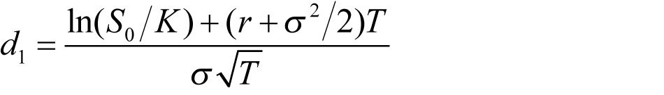 (1.3)
(1.3)
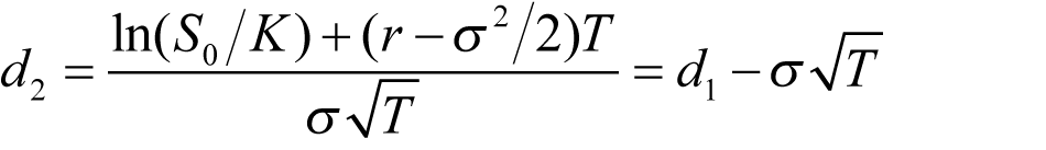 (1.4)
(1.4)
The variables c and p are the European call and put option price, S 0 is the stock price at time zero, K is the strike price, r is the continuously compounded risk-free interest rate, σ is the stock price volatility, and T is the time to maturity of the option, which is represented as: 3 months as 0.25, 6 months as 0.5, 1 year as 1.0.
The function N(x) in (1.1) and (1.2) is the cumulative probability distribution function of a standard normal distribution. The probability function of a standard normal distribution is given by the following equation, which is the first-order derivative of the standard normal distribution density function N(x) .
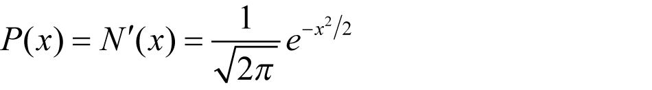 (1.5)
(1.5)
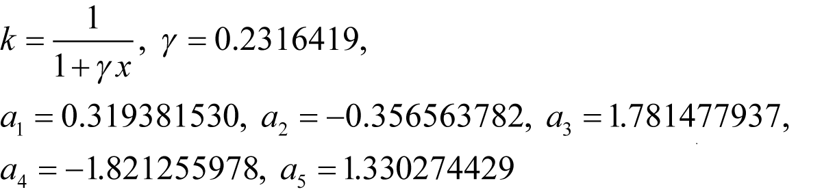
The only problem in implementing equations (1.1) and (1.2) is in computing the cumulative normal distribution function N(x) . This function can be approximated by a polynomial function that gives sixdecimal-place accuracy:
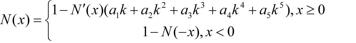 (1.6)
(1.6)
where:
The Black-Scholes model implemented in the PARSEC benchmark [Bienia11] is exactly as introduced in this section, and in the next section, the software implementation is from the PARSEC implementation with minor modifications [PARSEC] , the benchmark also comes with synthetic test data inputs (portfolio) based on replication of 1,000 real options. The benchmark is coded in C/C++ with default single precision floating point. The benchmark implementation offers thread-level parallelism with Pthreads, OpenMP and Intel TBB, and runs on Linux, Solaris 10, and Windows platforms. The benchmark can be compiled with GCC 4.3 and ICC 10.1 to run on SPARC, i386, X86_64 and ARM CPU architectures. 1
Software implementation of the Black-Scholes model
To compute a call or put option price in equations (1.1) and (1.2), we should first compute d1 and d2 in equations (1.3) and (1.4), and use the results to compute the standard normal distribution probability function in equation (1.5) and feed into the cumulative normal distribution function in equation (1.6), and then feed the results to compute the option price in equation (1.1) or (1.2). Following the flow of data, the model can be clearly divided into three sequential blocks: 1) D1D2, that is d1 from equation (1.3) and d2 from equation (1.4); 2) CNDF, the cumulative normal distribution function in equation (1.6); and 3) OP, the option price as in equation (1.1) and (1.2). The implementation of each function block with data inputs and outputs is shown below in sequence.
The D1D2 function takes five input parameters – spot price, strike price, interest rate, volatility and time-to-maturity – into computing equation (1.3) and (1.4), the results are returned into d1 and d2. (See Listing 1.)
typedef float fptype;
void D1D2(
//inputs
fptype spotprice,
fptype strike,
fptype rate,
fptype volatility,
fptype time,
//outputs
fptype* d1,
fptype* d2)
{
fptype xSqrtTime = sqrt(time);
fptype logValues = log(spotprice/strike);
fptype xPowerTerm = volatility * volatility;
xPowerTerm = xPowerTerm * 0.5;
fptype xD1 = rate + xPowerTerm;
xD1 = xD1 * time;
xD1 = xD1 + logValues;
fptype xDen = volatility * xSqrtTime;
xD1 = xD1/xDen;
fptype xD2 = xD1 xDen;
*d1 = xD1;
*d2 = xD2;
}
|
| Listing 1 |
The CNDF function implements cumulative normal distribution function in equation (1.5) and (1.6).The function takes d1 and d2 separately as its input and computes the cumulative normal distribution as its output (see Listing 2).
//Cumulative Normal Distribution Function
#define inv_sqrt_2xPI 0.39894228040143270286
fptype CNDF(fptype InputX)
{
int sign;
fptype OutputX;
fptype xInput;
fptype xNPrimeofX;
fptype expValues;
fptype xK2;
fptype xK2_2, xK2_3;
fptype xK2_4, xK2_5;
fptype xLocal, xLocal_1;
fptype xLocal_2, xLocal_3;
//Check for negative value of InputX
if (InputX<0.0){
InputX=-InputX;
sign=1;
}else
sign=0;
xInput=InputX;
// compute NPrimeX term common to both four &
// six decimal accuracy calcs
expValues = exp(-0.5f * InputX * InputX);
xNPrimeofX = expValues;
xNPrimeofX = xNPrimeofX * inv_sqrt_2xPI;
xK2 = 0.2316419 * xInput;
xK2 = 1.0 + xK2;
xK2 = 1.0/xK2;
xK2_2 = xK2 * xK2;
xK2_3 = xK2_2 * xK2;
xK2_4 = xK2_3 * xK2;
xK2_5 = xK2_4 * xK2;
xLocal_1 = xK2 * 0.319381530;
xLocal_2 = xK2_2 * (-0.356563782);
xLocal_3 = xK2_3 * 1.781477937;
xLocal_2 = xLocal_2 + xLocal_3;
xLocal_3 = xK2_4 * (-1.821255978);
xLocal_2 = xLocal_2 + xLocal_3;
xLocal_3 = xK2_5 * 1.330274429;
xLocal_2 = xLocal_2 + xLocal_3;
xLocal_1 = xLocal_2 + xLocal_1;
xLocal = xLocal_1 * xNPrimeofX;
xLocal = 1.0 – xLocal;
OutputX=xLocal;
if(sign){
OutputX = 1.0 OutputX;
}
return OutputX;
}
|
| Listing 2 |
The Black-Scholes equation takes seven input parameters, and computes the option price. The function implements equation (1.1) and (1.2) with calls to function D1D2 and CNDF (see Listing 3).
//OptionPrice
fptype BlackScholes(fptype spotprice,
fptype strike, fptype rate, fptype volatility,
fptype time, int otype, float timet)
{
fptype OptionPrice;
fptype FutureValueX;
fptype NofXd1;
fptype NofXd2;
fptype NegNofXd1;
fptype NegNofXd2;
fptype d1;
fptype d2;
//D1D2
D1D2(spotprice, strike, rate, volatility,
time, &d1, &d2);
//CNDF
NofXd1 = CNDF(d1);
NofXd2 = CNDF(d2);
//OP
FutureValueX = strike * (exp(-(rate)*(time)));
if (otype==0) {
OptionPrice = (spotprice * NofXd1)
(FutureValueX * NofXd2);
}else{
NegNofXd1 = (1.0 - NofXd1);
NegNofXd2 = (1.0 NofXd2);
OptionPrice = (FutureValueX * NegNofXd2)
(spotprice * NegNofXd1);
}
return OptionPrice;
}
|
| Listing 3 |
To run the multithreaded Black-Scholes application efficiently on a multicore CPU, the number of concurrent threads should match the number of cores to avoid unnecessary context switch, also use thread affinity to avoid unnecessary threads migration among different cores, and each thread should match its working sets size to the CPU cache and memory hierarchy. For example, one option input data entry can fit in one cache line of 64 bytes, a 64KB L1 cache can hold up to 1000 options, and while a 2MB L2 cache can hold up to a portfolio of 32 sets of 1000 options. As L1 access latency is a few (<10) cycles, L2 access latency is 10+ cycles, while L3 is usually shared among cores with 40 cycles access latency, and the off-chip memory takes more than 100 cycles to access, it makes sense to match the data sizes with the cache and memory hierarchy.
FPGA based accelerators for financial applications
There are a few companies offering FPGA-based accelerators for computing the Black-Scholes model and Monte-Carlo simulation for pricing options, such as Celoxica [ Morris07 ] and Maxeler [ Richards11 ].
Celoxica had implemented FPGA based acceleration technologies for European options pricing. They achieved 15 times speed-up over an existing server at full precision and have similar performance to GPU and Cell implementations as shown in the table below [ Morris07 ]. The accelerations achieved by FPGA, GPU and Cell BE are compared against the fully optimized C++ implementation running on a PC with a single core AMD 2.5GHz Opteron processor with 2 Gb of RAM and the Windows 2000 OS.
Table 1 shows a comparison of resource utilization, error and acceleration for different implementations of European option benchmark. In the table, LX/SX stands for two FPGA devices from the Xilinx Virtex 4 family, the LX160 and the SX55. The FPGA clock rates and accelerations are given for the LX device. Results indicated by * are estimates. The SX variant of the Virtex 4 family is significantly richer in DSP blocks resources, at the expense of fewer 4LUTS. The speed grade chosen for both devices was at the same -10 speed grade.
|
||||||||||||||||||||||||||||||||||||||||||||||||||||||||||||||||||||||||||||||||||||
| Table 1 | ||||||||||||||||||||||||||||||||||||||||||||||||||||||||||||||||||||||||||||||||||||
The component implemented in the FPGA is the computation unit for computing the following payoff equation (1.7). The computationally intensive component of computing the payoff equation is the Gaussian Random Number Generator, as Z n is generated by the Gaussian Random Number Generator (GRNG). The other components other than the GRNG for computing the above equation are just multipliers, adder, natural exponent, subtractor, max and accumulator.
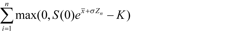 (1.7)
(1.7)
The payoff equation is implemented in HyperStreams that is built on the Handel-C 2 programming language. The data flow and the control flow of the implementation are separated, the data flow is programmed using the HyperStreams abstraction, and the control flow is programmed using traditional Handel-C syntax. The designs were synthesized using Celoxica DK5 and Xilinx ISE 9.1.
The block diagram in Figure 1 shows the portion of the European option-pricing algorithm implemented on FPGA, noting the separation of control and pipelined data flow. The parameters provided from the control flow to the data flow are fixed constants during the computation of the above equation and are therefore calculated in software.
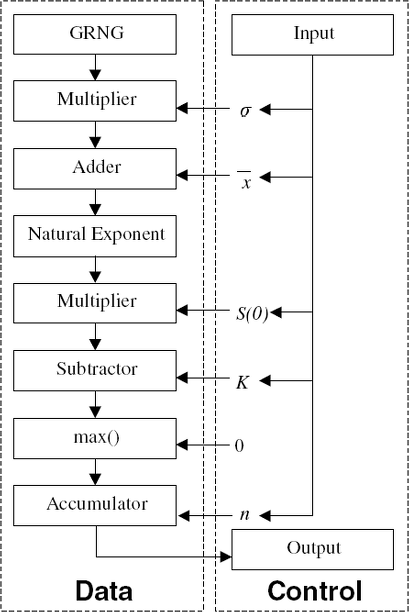
|
| Figure 1 |
As the FPGA designs are implemented in the high-level abstraction Handel-C programming language rather than implemented in RTL, it’s not a difficult task to implement the design in different flavours of floating point and fixed point. Balancing the resource utilization, performance and precision, the 32-bit fixed-point implementation offers the best results. The 18-bit fixed-point implementation offers 146 times performance acceleration but has 133 times worse precision compared to CPU as shown in Table 1, the single floating-point implementation offers 41 times acceleration but has 200 times downgrade on precision.
The power consumption and cost have not been taken into account when comparing the performances of different implementations. The Handel-C approach has a clear advantage on the time-to-market metric, as the five different flavours of floating point and fixed-point implementations only took two person days to implement. However, this approach doesn’t work out-of-the-box with legacy C/C++ code base, which limits its potential.
Maxeler worked with J.P. Morgan Quantitative Research to accelerate their tranche valuation [ Richards11 ]. The base correlation with stochastic recovery model is used to price and calculate risk for tranche-based products, such as vanilla tranches, bespoke tranches, n-th to default and CDO 2 . At its core, the model involves two key computationally intensive loops of constructing 1) the conditional survival probabilities using a Copula as shown in Equation (1.8) and 2) the probability of loss distribution using convolution as shown in Figure 2. Inside the convolution, FFT is used to evaluate the integral:
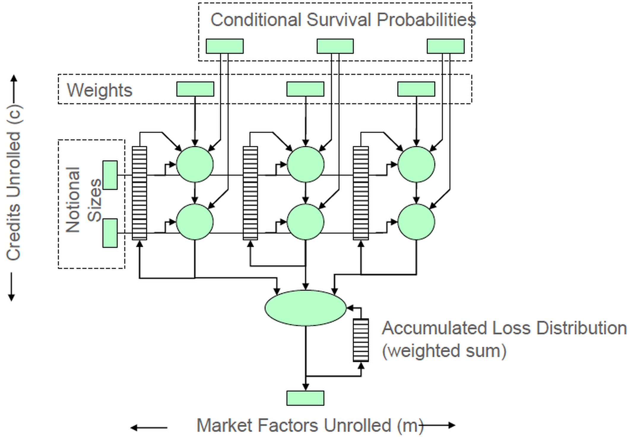
|
| Figure 2 |
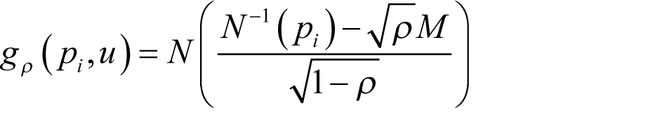 (1.8)
(1.8)
where g p is the conditional survival probability for this name, p i is the unconditional survival probability for this name, ρ is the correlation and M is the market factor.
The valuation of tranched CDOs can be expressed in flattened C code as below after removing all use of classes, templates and other C++ features in order to simplify parallelization. The Copula takes 23% of execution time and the Convolution takes 75% of execution time in CPU. (Listing 4.)
for i in 0 ... markets-1
for j in 0 ... names-1
prob = cum_norm((inv_norm(Q[j])
sqrt(p)M)/sqrt(1-p);
loss = calc_loss(prob,Q2[j],
RR[j],RM[j])*notional[j];
n = integer(loss);
L = fractional(loss);
for k in 0 ... bins-1
if j == 0
dist[k] = k == 0 ? 1.0 : 0.0;
dist[k] = dist[k]*(1-prob) +
dist[k-n]*prob*(1-L) +
dist[k-n-1]*prob*L;
ifj==credits -1
final_dist[k] += weight[i] * dist[k];
end # for k
end # for j
end # for i
|
| Listing 4 |
After offloading the computation of Copula and Convolution onto the FPGA from the CPU, a single FPGA prices a complex trade 134 times faster than a single CPU. As a result, end-to-end time to price global credit hybrids portfolio once reduced to ~125 seconds with pure FPGA time of ~2 seconds to price ~30,000 tranches and total compute time of ~30 seconds. End-to-end time for pointwise credit deltas on global credit hybrids portfolio reduced to ~238 seconds with pure FPGA time of ~12 seconds, using a 40-node FPGA machine. End-to-end time to run multiple trading/risk scenarios for desk reduced to ~320 seconds with results accurate to within $5 across global portfolio, while it’s not previously possible to run such scenarios multiple times within a single trading day.
In addition to acceleration, the FPGA based solutions have predictable performance for computation and data I/O, as FPGAs are statically scheduled and with no cache involved. However, JPMorgan took a 20% stake in Maxeler, which potentially limits its adoption in other financial institutions.
FPGA based high performance computing for financial applications
Tandon [ Tandon03 ] completed a Master’s Thesis on A Programmable Architecture for Real-Time Derivative Trading , which he implements the Black-Scholes European Option Pricing model on FPGA, simulated ARM processor and Mathematica, which is used as the reference platform, and compares their performance acceleration and accuracy. The results are shown in Table 2.
|
||||||||||||
| Table 2 |
In Table 2, time per iteration means the time used to compute either a call or put option price using the Black-Scholes model given a set of input data. The Reference Mathematica test is conducted on Mathematica 5.0 on an Intel Pentium 4 processor at 2.53 GHz. The Black-Scholes model is implemented in Mathematica using some of its library functions that are assumed to have suitable optimizations or approximations. Floating point is used in this implementation, but the thesis doesn’t tell whether it being single or double floating point. The simulated ARM processor is done on a simulated ARM7TDMI processor running at 200MHz, the Black-Scholes model is implemented in ANSI-C with floating point and targets towards an ARM7 processor. The simulated ARM7TDMI simulates all floating-point computations within the processor itself rather than having a dedicated floating-point unit. The FPGA based implementation coded in VHDL 3 has not been synthesized successfully due to it being a purely floating-point computation and the IEEE math library that is used for the floating-point computations is designed for simulation only. However, modifications have been made to the design to make it integer based, the performance numbers are drawn from the integer-based implementation of the Black-Scholes model on a Virtex-II Pro FPGA. The 50ns time per iteration number shown in the table, however, is not measured from real experimental hardware rather it is an estimated number inferred from the synthesis report of the design. The downgrade from floating point to integer-based implementation significantly undermines the accuracy.
The challenges faced in the Black-Scholes model FPGA implementation using floating point in the thesis however points out that a fixed-point implementation of the Black-Scholes model on FPGA is more favourable considering the manpower required to implemented the floating-point capability and the accuracy tradeoff between floating point and fixed point.
It is also pointed out that financial models are very heavily dependent on calculus, probability, statistics and other branches of Mathematics, a logic library which has RTL implementations of some fundamental mathematical functions would be very useful, such as, integration, higher order derivation, random number generation, statistical and stochastic modelling, vector calculus, trigonometric functions and logarithmic functions. Although the idea is constructive for putting more financial models on FPGAs easily, it should be noted that integration is not necessary for calculating cumulative normal distribution function in the Black-Scholes model, as a polynomial approximation that gives six-decimal-place accuracy is given in [ Hull06 ].
Black-Scholes hardware design
The Black-Scholes model can be similarly implemented in three hardware modules: D1D2, CNDF and OptionPrice, as shown in Figure 3. D1D2 module computes Equations (1.3) and (1.4); it takes five data inputs and then feed the two outputs to the two parallel CNDF modules. CNDF (Cumulative Normal Distribution function) module computes Equation (1.5) and (1.6); it takes the input from D1D2 and feeds the output to OptionPrice module. OptionPrice computes Equation (1.1) and (1.2); it takes four data inputs, one option type control signal and two data feeds from CNDF modules, the module gives the price of the option as the output. The implementation takes 25 clock cycles to compute the option price based on the five data inputs and one option type control input, with each arithmetic unit taking only one cycle to compute for simplicity 4 . The data path resource utilization and the time delay of each module are summarized in Table 3.
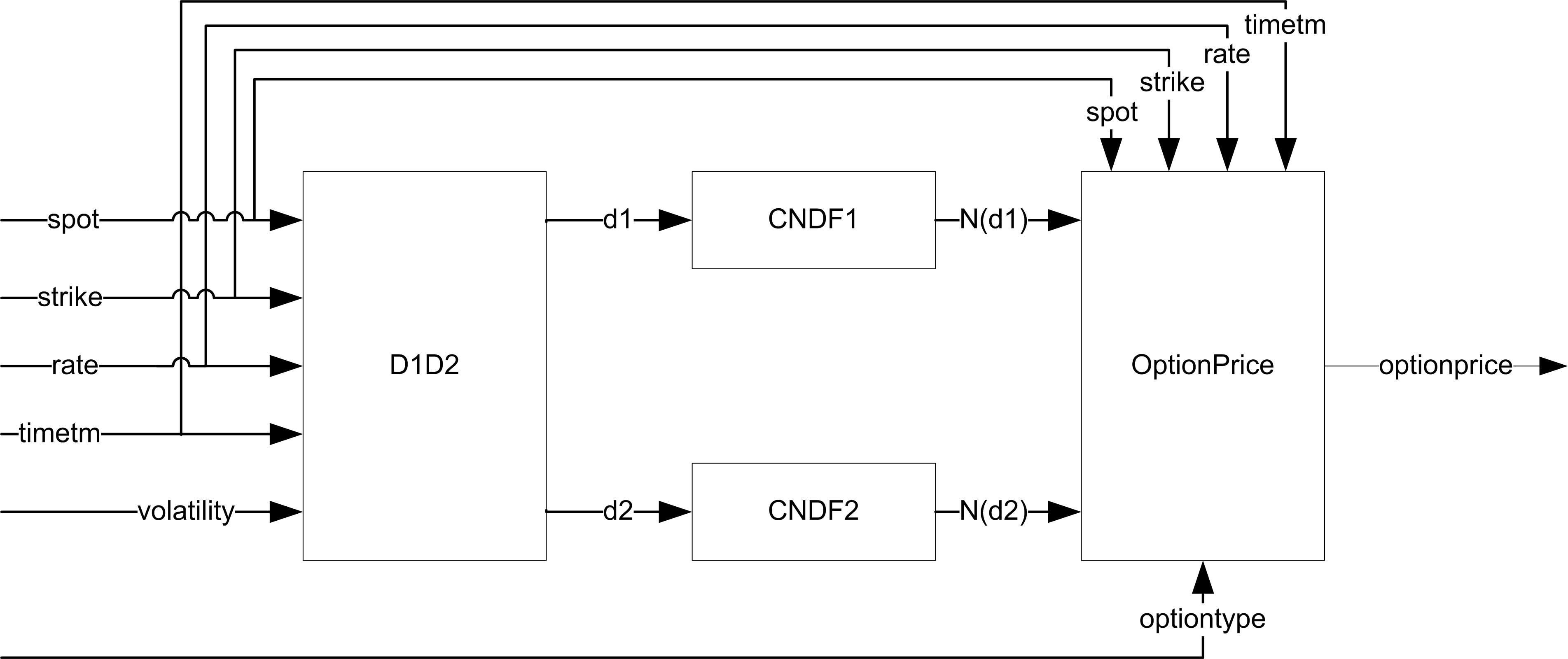
|
| Figure 3 |
|
|||||||||||||||||||||||||||||||||||||||||||||||||||||
| Table 3 | |||||||||||||||||||||||||||||||||||||||||||||||||||||
The resource utilization count assumes each hardware arithmetic unit is shared among D1D2, CNDF and OptionPrice blocks where possible. In a fully pipelined implementation, we would see at the bottom row the sum of each column rather than the maximum of each column, for example, in column
+
, it would be three
+
hardware arithmetic units rather than one unit to be needed for the implementation. The clock cycle count can be seen visually in the block diagrams as shown in Figure 4, Figure 5, Figure 6, each horizontal level represents one cycle delay.
In the following sections, the implementation details of D1D2, CNDF and OptionPrice blocks are explained.
D1D2 block design
This block takes 7 cycles to execute, it has 1 add unit, 1 subtract unit, 2 multiply units, 1 divide unit, 1 square root unit and 1 logarithm unit, as shown in Figure 4. The inputs to the block are spot price, strike price, time to mature, volatility and interest rate, which are shown on the top of Figure 4, and the outputs of the block are d1 and d2, which are shown at the bottom of Figure 4. The input from the right of the block diagram is the control signal to the data path; it is a constant in this case.
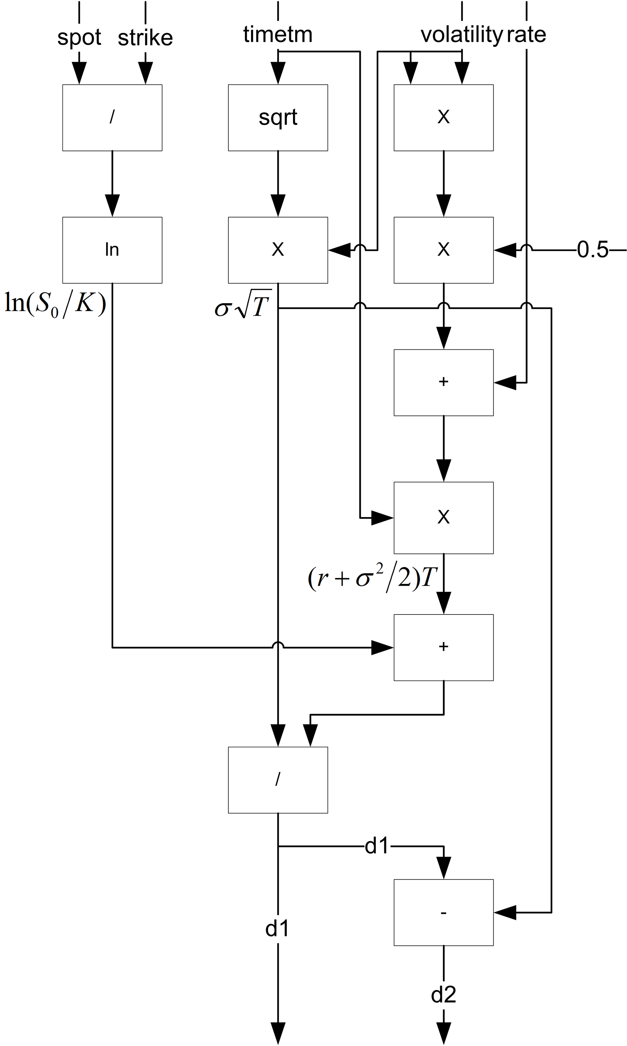
|
| Figure 4 |
CNDF block design
This block takes 12 cycles to execute, it has 1 add unit, 1 subtract unit, 3 multiply units, 1 divide unit, 1 exponential unit, as shown in Figure 5. The inputs on the top of the block diagram are inputs to the module and the outputs at the bottom of the block diagram are the outputs of the module. The inputs from the right of the diagram are control signals to the data path.
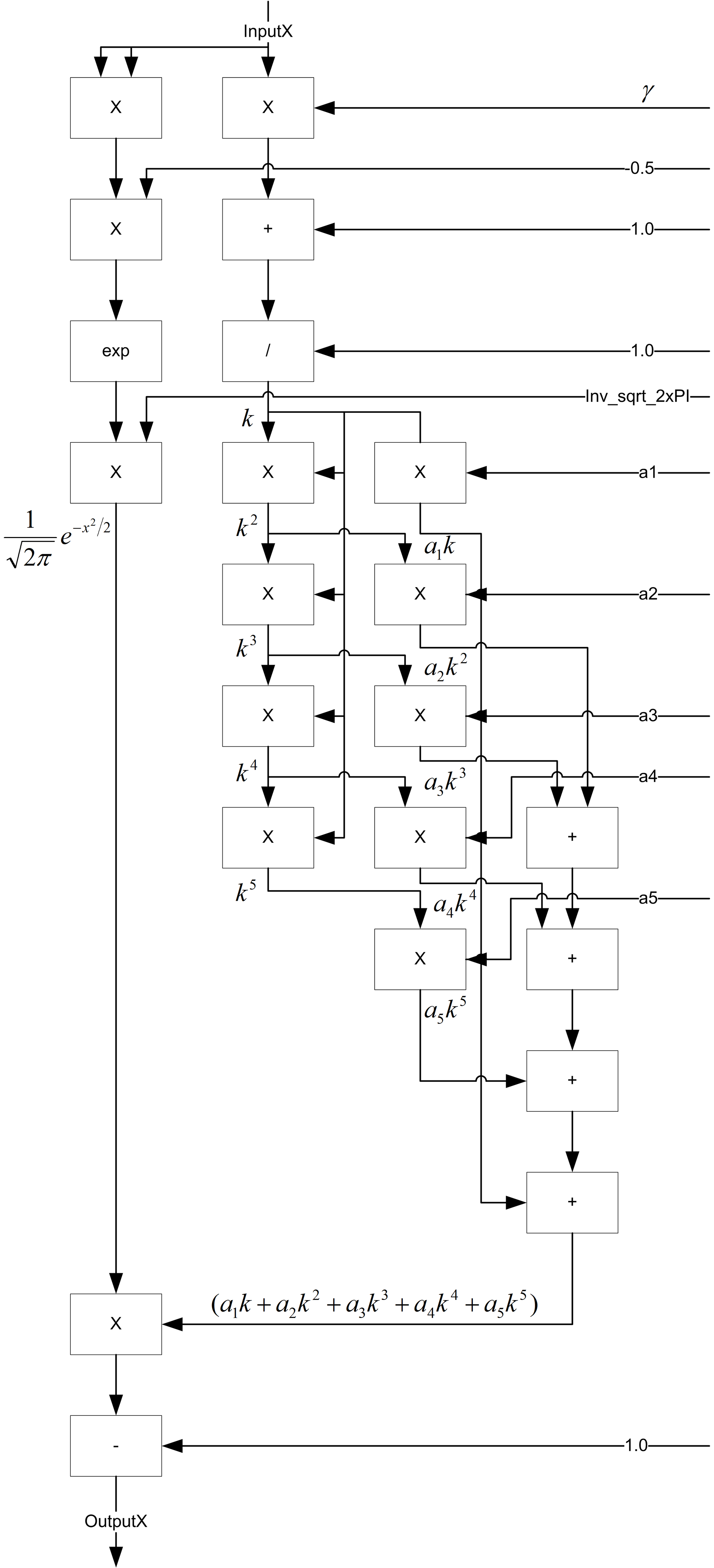
|
| Figure 5 |
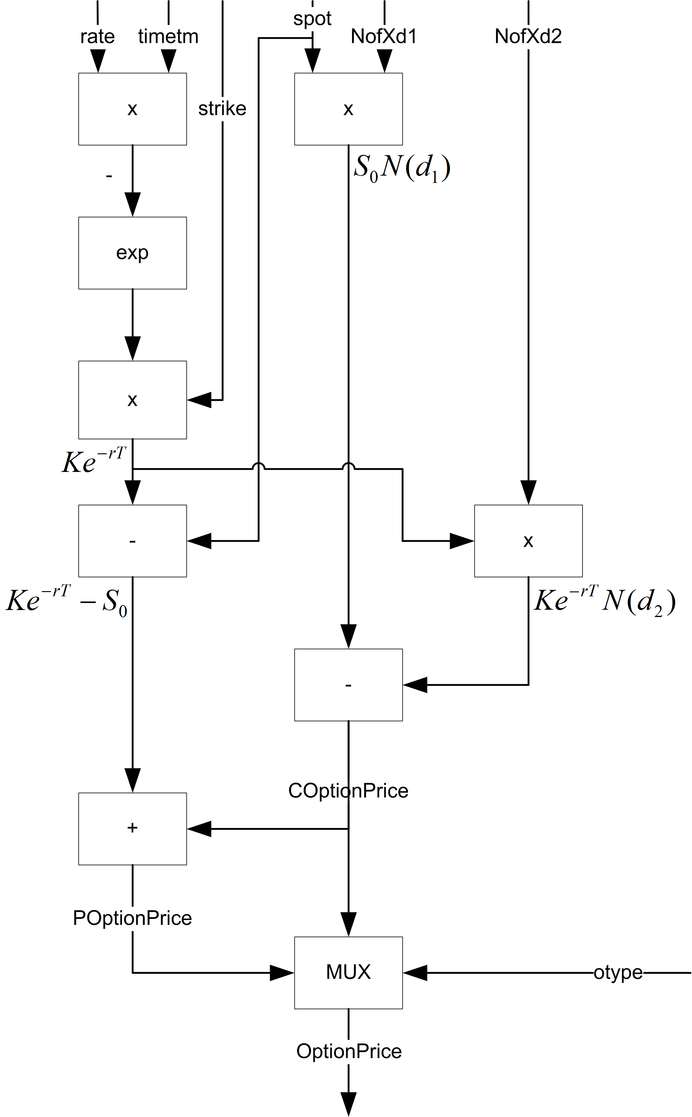
OptionPrice block design
This block takes 6 cycles to execute, it has 1 add unit, 1 subtract unit, 2 multiply units and 1exponential unit as shown in Figure 6. The inputs on the top of the diagram are inputs to the module and the outputs at the bottom of the diagram are the outputs of the module. The inputs from the right of the diagram are control signals to the data path.
|
| Figure 6 |
Black-Scholes hardware implementation
The hardware implementation is based on single precision floating point, as the baseline implementation in PARSEC is in single precision floating point. The decision to implement the model whether in single-precision floating point or 32-bit/18-bit fixed point depends on the efforts to implement, the logic resource requirement, and the speed of acceleration and the accuracy. The floating-point arithmetic units make use of the components from the Synopsys DesignWare floating-point datapath library [ Synopsys ] and the Synopsys Synplify Premier 2010.09 for FPGA implementation. DesignWare floating-point library contains all the components needed to implement the floating point arithmetic functions of +, -, *, /, sqrt, exp and ln in the Black-Scholes model. The Synopsys DesignWare library is optimized for ASIC implementation rather than FPGA, though the design efforts are minimal, the area of the design is huge when synthesized to FPGA.
An area optimized floating point library of square root, logarithm and exponential components was later developed specifically for FPGA, which showed significant improvements in implementation area and fits the whole design onto a tiny Xilinx Spartan 3A FPGA as shown in Table 4. The Add/Sub/Mult/Div uses the Xilinx floating-point operators. The square root and logarithm are implemented CORDIC rolled [ Wikipedia11 ], while the exponential is implemented using table lookup.
|
|||||||||||||||||||||
| Table 4 |
Conclusion
Derivatives pricing is at the core of financial trading and risk management. As shown in [Richards11] , FPGA offers the opportunity for real-time risk visibility to monitoring and controlling financial risk of complex derivatives that are not possible on CPUs.
The intention for this article is to show software engineers how an algorithm can be implemented in software and hardware. As each arithmetic unit matches to a hardware component, so the software implementation is intentionally coded like how it should be implemented in hardware. The idea is that it should be very easy to match the hardware block diagrams to the corresponding software function implementations.
The Black-Scholes model serves as a baseline of all financial models for pricing derivatives, most of these financial models rely on the same floating point computations of the seven basic arithmetic operations: add, subtract, multiply, divide, square root, logarithm and exponential. The intention is that it should be very easy to move from Black-Scholes to another financial model, such as HJM for pricing swaptions or base correlation with stochastic recovery for pricing tranches.
References
[Bienia11] Christian Bienia, Benchmarking Modern Multiprocessors , Princeton University, New Jersey, PhD Thesis 2011.
[Hull06] John C. Hull, Options, futures and other derivatives , 6th ed. New Jersey, U.S.A: Prentice-Hall, 2006, pp. 295-298.
[Morris07] Gareth W. Morris and Matt Aubury, ‘Design Space Exploration of the European Option Benchmark Using HyperStreams’ in Field Programmable Logic and Applications (FPL), 2007., Amsterdam, 2007, pp. 5-10.
[PARSEC] Source code available at: http://parsec.cs.princeton.edu/
[Richards11] Peter Richards and Stephen Weston. (2011, May) Stanford EE Computer Systems Colloquium.[Online]. http://www.stanford.edu/class/ee380/Abstracts/110511.html
[Synopsys] Synopsys Inc. ‘Datapath – Floating Point Overview.’
[Tandon03] Sachin Tandon, A Programmable Architecture for Real-Time Derivative Trading , Computer Science, University of Edinburgh, Edinburgh, MSc Thesis 2003.
[Wikipedia11] Wikipedia. (2011, Feb) http://en.wikipedia.org/wiki/CORDIC.
- The PARSEC benchmark also includes another financial analysis application, the HJM (Heath-Jarrow-Morton) model to price swaptions, implemented in C++ with multithreading support for Pthreads and Intel TBB on Linux and Solaris 10 platforms. Due to the data-level parallelization of the workload, the performance scales well with the number of available cores on a CPU.
- Handel-C is a programming language and is not a Hardware Description Language (HDL) for compiling programs into hardware images of FPGAs or ASICs. It is a rich subset of C, with non-standard extensions to control hardware instantiation and parallelism.
- VHSIC Hardware Description Language
- The one cycle implementation is not area efficient and cost effective, the more complex arithmetic units, such as divide, square root, and logarithm and exponential, take more than 20 cycles to compute in practice.