We’re still trying to find a good way to approach numerical computing. Richard Harris tries to get as close as possible.
We began this arc of articles with a potted history of the differential calculus; from its origin in the infinitesimals of the 17 th century, through its formalisation with Analysis in the 19 th and the eventual bringing of rigour to the infinitesimals of the 20 th .
We then covered Taylor’s theorem which states that, for a function f

where f' ( x ) stands for the first derivative of f at x , f" ( x ) for the second and f ( n )( x ) for the n th with the convention that the 0 th derivative of a function is the function itself.
We went on to use it in a comprehensive analysis of finite difference approximations to the derivative in which we discovered that their accuracy is a balance between approximation error and cancellation error, that it always depends upon the unknown behaviour of higher derivatives of the function and that improving accuracy by increasing the number of terms in the approximation is a rather tedious exercise.
Of these issues, the last rather stands out; from tedious to automated is often but a simple matter of programming. Of course we shall first have to figure out an algorithm, but fortunately we shall be able to do so with relatively ease using, you guessed it, Taylor’s theorem.
Finding the truncated Taylor series
The first step is to truncate the series to the first n terms and make the simple substitution of y for x + δ , giving

or

to n th order in y - x .
Next we evaluate f at n points in the vicinity of x , say y 1 to y n , yielding

Now the only unknowns in these equations are the derivatives of f so they are effectively a set of simultaneous linear equations of those derivatives and can be solved using the standard technique of eliminating variables.
By way of an example, consider the equations

To recover the value of x , we begin by eliminating z from the set of equations which we can do with

Next, we eliminate y with

and hence x is equal to 1.
At each step in this process we transform a system of n equations of n unknowns into a system of n -1 equations of n -1 unknowns and it is therefore supremely well suited to a recursive implementation, as shown in listing 1.
template<class T>
T
solve_impl(std::vector<std::vector<T> > &lhs,
           std::vector<T> &rhs,
           const size_t n)
{
  for(size_t i=0;i!=n;++i)
  {
    for(size_t j=0;j!=n;++j)
    {
      lhs[i][j] -= lhs[i][n]*lhs[n][j]/lhs[n][n];
    }
    rhs[i] -= lhs[i][n]*rhs[n]/lhs[n][n];
  }
  return n!=0 ? solve_impl(lhs, rhs, n-1)
              : rhs[0]/lhs[0][0];
}
template<class T>
T
solve(std::vector<std::vector<T> > lhs,
      std::vector<T> rhs)
{
  if(rhs.empty())
     throw std::invalid_argument("");
  if(lhs.size()!=rhs.size())
     throw std::invalid_argument("");
  for(size_t i=0;i!=lhs.size();++i)
  {
    if(lhs[i].size()!=rhs.size())
       throw std::invalid_argument("");
  }
  return solve_impl(lhs, rhs, rhs.size()-1);
}
|
| Listing 1 |
The first thing we need to do before we can use this to compute the derivative of a function is to decide what values we should choose for each y i .
We can do this by extrapolating our analysis of finite differences; for an n th order approximation, we should choose

to yield an error of order
 .
.
Following a similar argument to that we used to choose the values of δ for our finite difference approximations, we shall choose

Polynomial derivative approximation
Listing 2 gives the class definition for a polynomial derivative approximation function object based upon these observations.
template<class F>
class polynomial_derivative
{
public:
  typedef F function_type;
  typedef typename F::argument_type argument_type;
  typedef typename F::result_type result_type;

  polynomial_derivative(const function_type &f,
                        unsigned long n);

  result_type operator()(
     const argument_type &x) const;

private:
  function_type f_;
  unsigned long n_;
  argument_type ef_;
};
|
| Listing 2 |
The constructor is relatively straightforward, as shown in listing 3. Note that the
epsilon
function is represented here by the typesetter-friendly abbreviation
eps
<T>
).
template<class F>
polynomial_derivative<F>::polynomial_derivative(
  const function_type &f, const unsigned long n)
: f_(f),
  n_(n),
  ef_(pow(argument_type(n+1)*
          eps<argument_type>(),
          argument_type(1)/argument_type(n+1)))
{
  if(n==0) throw std::invalid_argument("");
}
|
| Listing 3 |
Once again we assume that we have specialisations of both
std::numeric_limits
and
pow
for the function’s argument type.
Listing 4 provide the definition of the function call operator.
template<class F>
typename polynomial_derivative<F>::result_type
polynomial_derivative<F>::operator()(
   const argument_type &x) const
{
  std::vector<std::vector<result_type> >
     lhs(n, std::vector<result_type>(n));
  std::vector<result_type> rhs(n);
  const argument_type abs_x =
     (x>argument_type(0)) ? x : -x;
  const result_type fx = f_(x);
  for(size_t i=0;i!=n_;++i)
  {
    const argument_type y =
      x +argument_type(i+1)*ef_*(
         abs_x+argument_type(1));
    result_type fac(1);
    for(size_t j=0;j!=n_;++j)
    {
      fac *= result_type(j+1);
      const result_type dn = pow(result_type(y-x),
                                 result_type(j+1));
      lhs[i][j] = dn/fac;
    }
    rhs[i] = f_(y)-f_(x);
  }
  return solve_impl(lhs, rhs, n_-1);
}
|
| Listing 4 |
Note that if the argument and result types are different we shall very likely introduce a potential source of numerical error. Consequently we should ideally only use this class for functions with the same argument and result types.
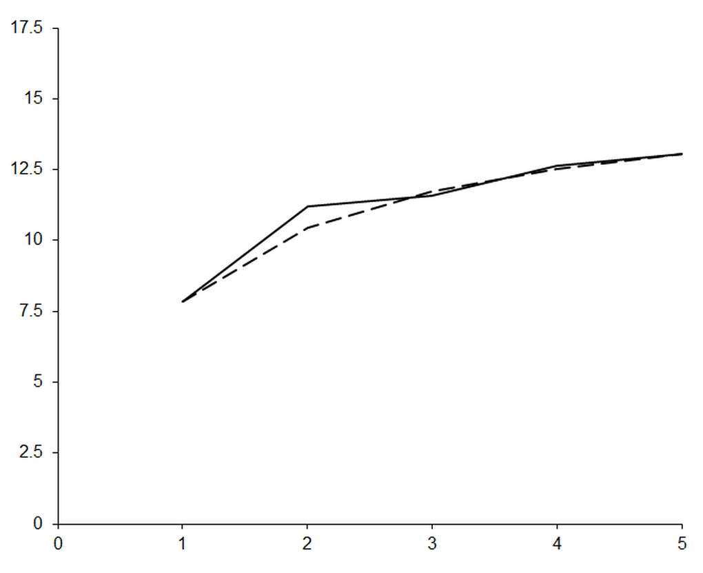
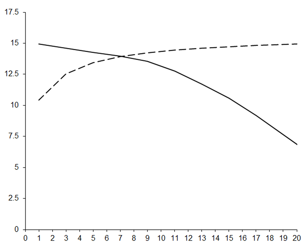
Figure 1 plots the negation of the base 10 logarithm of the absolute error in this approximate derivative of the exponential function at zero, equivalent to the number of accurate decimal places, against the order of the approximation. The dashed line shows the negation of the base 10 logarithm of the expected order of the error in the approximation,
 .
.
|
| Figure 1 |
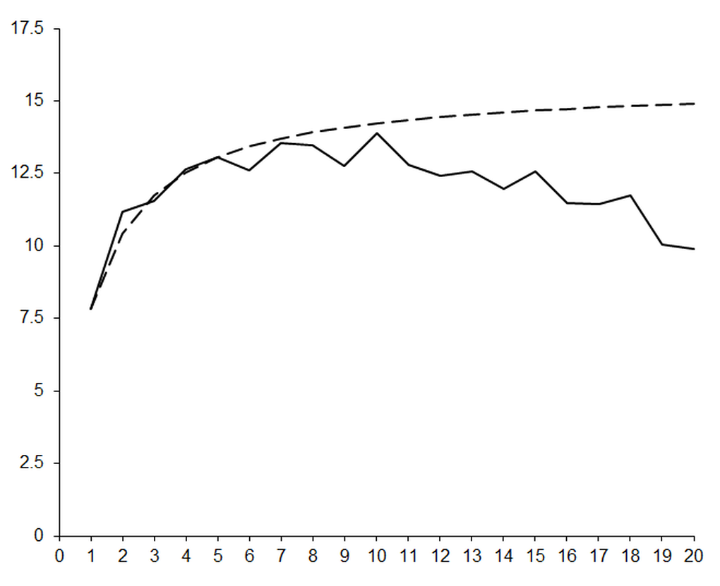
This certainly seems to be a step in the right direction; as we increase the order of our polynomials the number of accurate digits grow exactly as expected. We should consequently expect that by increasing the order of the polynomials we should bring the error arbitrarily close to ε , as shown in figure 2.
|
| Figure 2 |
Something has gone horribly wrong! As we expend ever increasing effort in improving the approximation, the errors are getting worse .
The reason for this disastrous result should be apparent if you spend a little time studying our simultaneous equation solver. We are performing large numbers of subtractions and divisions; if this doesn’t scream cancellation error at you then you haven’t been paying attention!
We can demonstrate the problem quite neatly if we use interval arithmetic to keep track of floating point errors. You will recall with interval arithmetic we keep track of an upper and lower bound on a floating point calculation by choosing the most pessimistic bounds on the result of an operation and then rounding the lower bound down and the upper bound up.
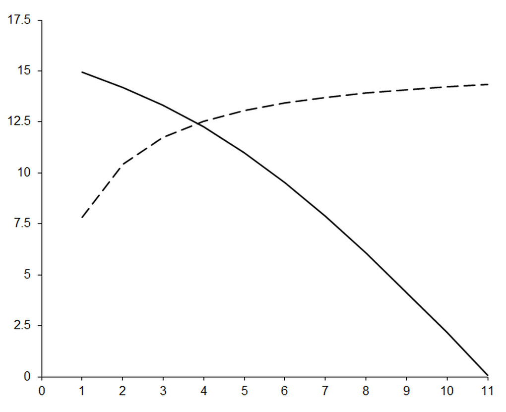
Figure 3 plots the approximate number of decimal places of agreement between the upper and lower bound of the interval result of the approximation as a solid line and the expected order of the error as a dashed line.
|
| Figure 3 |
This clearly shows that our higher order polynomial approximations are suffering from massive loss of precision. We can’t plot results above 11 th order since the intervals are infinite; these calculations have effectively lost all digits of precision.
Note that the intersection of the two curves provides a reasonable choice of 4 for the polynomial order we should use to calculate this specific derivative.
Improving the algorithm
Our algorithm is, in fact, the first step in the Gaussian elimination technique for solving simultaneous linear equations. The second stage is that of back-substitution during which the remaining unknowns are recovered by recursively substituting back to the equations each unknown as it is revealed. We are able to skip this step because we are only interested in one of the unknowns.
However, as it stands, our algorithm is not particularly well implemented.
Firstly, if every value in a column in the left hand side is zero, an unlikely but not impossible prospect, we shall end up dividing zero by zero.
Secondly, and more importantly, by eliminating rows in reverse order of the magnitude of δ , we risk dividing by small values and unnecessarily amplifying rounding errors; a far better scheme is to choose the row with the largest absolute value in the column we are eliminating.
Listing 5 provides a more robust implementation of our simultaneous equation solver that corrects these weaknesses.
template<class T>
T
solve_impl(std::vector<std::vector<T> > &lhs,
           std::vector<T> &rhs,
           const size_t n)
{
  T abs_nn =
     lhs[n][n]>T(0) ? lhs[n][n] : -lhs[n][n];
  for(size_t i=0;i!=n;++i)
  {
    const T abs_in =
       lhs[i][n]>T(0) ? lhs[i][n] : -lhs[i][n];
    if(abs_in>abs_nn)
    {
      abs_nn = abs_in;
      std::swap(lhs[i], lhs[n]);
      std::swap(rhs[i], rhs[n]);
    }
  }
  if(abs_nn>T(0))
  {
    for(size_t i=0;i!=n;++i)
    {
      for(size_t j=0;j!=n;++j)
      {
        lhs[i][j] -=
           lhs[i][n]*lhs[n][j]/lhs[n][n];
      }
      rhs[i] -= lhs[i][n]*rhs[n]/lhs[n][n];
    }
  }
  return n!=0 ? solve_impl(lhs, rhs, n-1) :
     rhs[0]/lhs[0][0];
}
|
| Listing 5 |
Unfortunately, whilst this certainly improves the general stability of our algorithm, it does not make much difference to its accuracy.
A more effective approach is to try and minimise the number of arithmetic operations we require for our algorithm. We can do this by exploiting the very same observation that led us to the symmetric finite difference; that the difference between a pair of evaluations of the function an equal distance above and below x depends only on the odd ordered derivatives.

This will yield an error of the same order as our first implementation with approximately half the number of simultaneous equations and consequently roughly one eighth of the arithmetic operations.
Listing 6 shows the required changes in the
polynomial_derivative
member functions.
template<class F>
polynomial_derivative<F>::polynomial_derivative(
  const function_type &f,
  const unsigned long n)
: f_(f), n_(n),
  ef_(pow(argument_type(2*n+1)
      *eps<argument_type>(),
      argument_type(1)/argument_type(2*n+1))),
  lhs_(n, std::vector<result_type>(n)),
  rhs_(n)
{
  if(n==0) throw std::invalid_argument("");
}
template<class F>
typename polynomial_derivative<F>::result_type
polynomial_derivative<F>::operator()(
   const argument_type &x) const
{
  const argument_type abs_x =
     (x> result_type(0)) ? x : -x;
  for(size_t i=0;i!=n_;++i)
  {
    const argument_type y =
       abs_x + argument_type(i+1)*ef_*(
       abs_x+argument_type(1));
    const argument_type d = y-abs_x;
    result_type fac(1);
    for(size_t j=0;j!=n_;++j)
    {
      const result_type dn =
         pow(result_type(d), result_type(2*j+1));
      lhs_[i][j] = dn/fac;
      fac *=
         result_type(2*j+2) * result_type(2*j+3);
    }
    rhs_[i] = (f_(x+d)-f_(x-d)) / result_type(2);
  }
  return solve_impl(lhs_, rhs_, n_-1);
}
|
| Listing 6 |
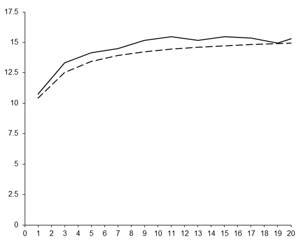
Figure 4 illustrates the impact upon the number of accurate digits in the results of our improved approximations.
|
| Figure 4 |
Clearly, this is far better than our first attempt; the observed error is consistently smaller than expected. However, on performing the calculation using interval arithmetic, we find that we are still restricted by cancellation error, as shown in figure 5.
|
| Figure 5 |
If we choose the point at which the observed cancellation error crosses the expected error, shown as a dashed line, we should choose a 7 th order polynomial, corresponding again to 4 simultaneous equations.
These polynomial approximation algorithms are certainly an improvement upon finite differences since we have automated the annoying process of working out the formulae. However, we are still clearly constrained by the trade off between approximation and cancellation error.
This problem is fundamental to the basic approach of these algorithms; computing the coefficients of the Taylor series by solving simultaneous equations is inherently numerically unstable.
To understand why, it is illuminating to recast the problem as one of linear algebra.
A problem of linear algebra
By the rules of matrix and vector arithmetic we have, for a matrix M and vectors v and w

where subscripts i , j of a matrix denote the j th column of the i th row, a subscript i of a vector denotes its i th element and the capital sigma denotes the sum of the expression to its right for every valid value of the symbol beneath it.
We can consequently represent the simultaneous equations of our improved algorithm with a single matrix-vector equation if we choose the elements of M , v and w such that

for i and j from one up to and including n .
Those matrices with the same number of rows and columns, say n , whose elements are equal to one if the column index is equal to the row index and zero otherwise we call identity matrices, denoted by I . These have the property that for all vectors v with n elements

If we can find a matrix M -1 such that

known as the inverse of M , we have

Our algorithm is therefore, in some sense, equivalent to inverting the matrix M .
That this can be a source of errors is best demonstrated by considering the geometric interpretation of linear algebra in which we treat a vector as Cartesian coordinates identifying a point.
For example, in two dimensions we have

Hence every two by two matrix represents a function that takes a point in the plane and returns another point in the plane.
If it so happens that c ÷ a equals d ÷ b then we are in trouble since the two dimensional plane is transformed into a one dimensional line.
For example, if

then

Given the result of such a function there is no possible way to identify which of the infinite number of inputs might have yielded it.
Such matrices are known as singular matrices and attempting to invert them is analogous to dividing by zero. They are not, however, the cause of our problems. Rather, we are troubled by matrices that are nearly singular.
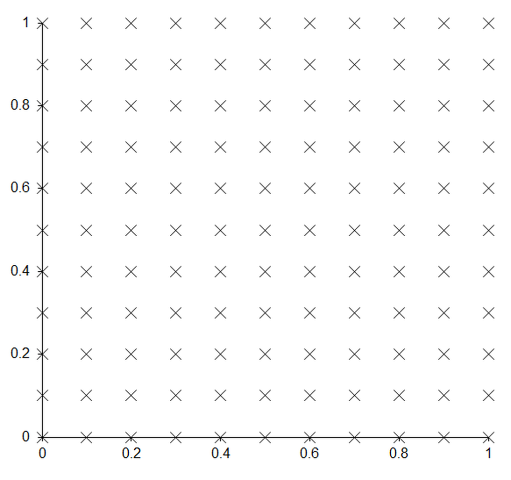
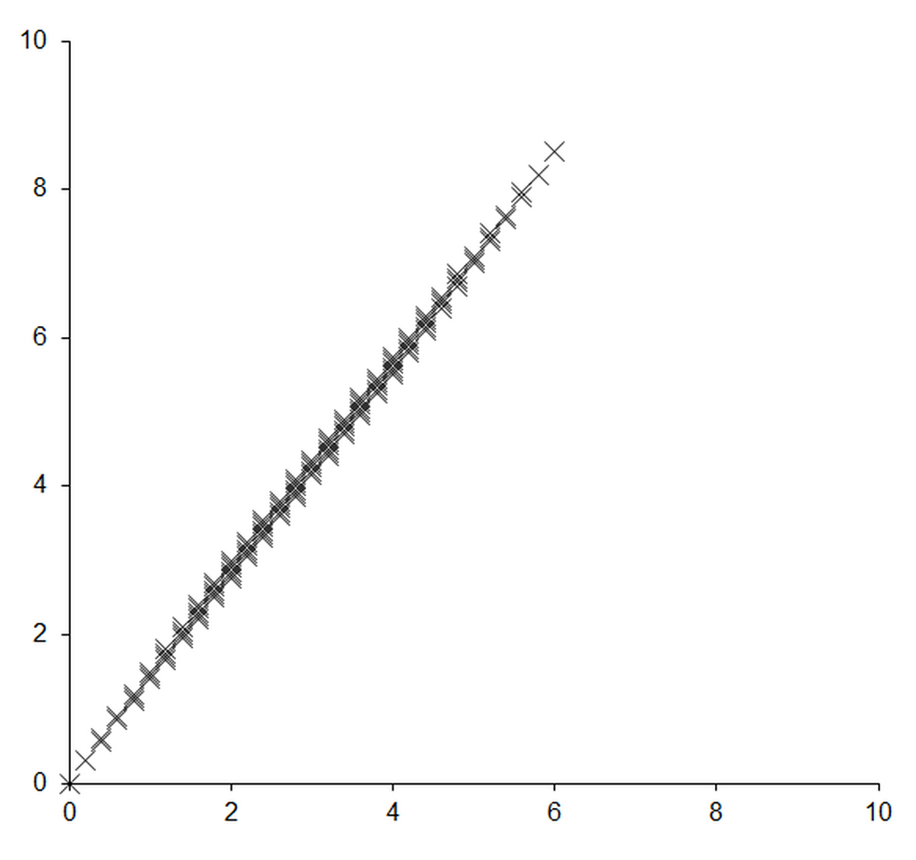
To understand what this means, consider the two dimensional matrix

Figure 6 shows the result of multiplying a set of equally spaced points on the unit square by this matrix. The points clearly end up very close to a straight line rather than exactly upon one.
|
|
| Figure 6 |
To a mathematician, who is equipped with the infinitely precise real numbers, this isn’t really a problem. To a computer programmer, who is not, it causes no end of trouble. One dimension of the original data has been compressed to small deviations from the line. These deviations are represented by the least significant digits in the coordinates of the points and much information about the original positions is necessarily rounded off and lost. Any attempt to reverse the process cannot recover the original positions of the points with very much accuracy; cancellation error is the inevitable consequence.
That our approximations should lead to such matrices becomes clear when you consider the right hand side of the equation. We choose δ as small as possible in order to minimise approximation error with the result that the function is evaluated at a set of relatively close points. These evaluations will generally lie close to a straight line since the behaviour of the function will largely be governed by the first two terms in its Taylor series expansion.
Unfortunately, the approach we have used to mitigate cancellation error is horribly inefficient since we must solve a new system of simultaneous equations each time we increase the order of the approximating polynomials.
The question is whether there is there a better way?
Ridders’ algorithm
The trick is to turn the problem on its head; rather than approximate the function with a polynomial and use its coefficients to approximate the derivative we treat the symmetric finite difference itself as a function of δ and approximate it with a polynomial.
Specifically, if we define

and we vigorously wave our hands, we have

Now, if we approximate
 with an
n
th
order polynomial
with an
n
th
order polynomial
 then we can approximate the derivative of
f
by evaluating it at 0
then we can approximate the derivative of
f
by evaluating it at 0

We could try to find an explicit formula for
 by evaluating
 at
n
non-zero values of
δ
and solving the resulting set of linear equations, as we did in our first polynomial algorithm, but we would end up with the same inefficiency as before when seeking the optimal order.
at
n
non-zero values of
δ
and solving the resulting set of linear equations, as we did in our first polynomial algorithm, but we would end up with the same inefficiency as before when seeking the optimal order.
Ridders’ algorithm [ Ridders82 ] avoids this problem by evaluating the polynomial at zero without explicitly computing its coefficients. That this is even possible might seem a little unlikely, but nevertheless there is more than one way to do so.
Neville’s algorithm
We can easily compute the value of the polynomial that passes through a pair of points, trivially a straight line, without explicitly computing its coefficients with a kind of pro-rata formula.
Given a pair of points ( x 0 , y 0 ) and ( x 1 , y 1 ), the line that passes through them consists of the points ( x , y ) where

This can be rearranged to yield an equation for the line

Neville’s algorithm, described in Numerical Recipes in C [ Press92 ], generalises this approach to any number of points, or equivalently any order of polynomial, and takes the form of a recursive set of formulae.
Given a set of n points ( x i , y i ) and a value x at which we wish to evaluate the polynomial that passes through them, we define the formulae

from which we retrieve the value of the polynomial at x with p 1 , n ( x ).
If we arrange the formulae in a triangular tableau, we can see that as the calculation progresses each value is derived from the pair above and below to its left.

This shows why this algorithm is so useful; adding a new point introduces a new set of values without affecting those already calculated. We can consequently increase the order of the polynomial approximation without having to recalculate the entire tableau.
Further noting that we actually only really need the lower diagonal values when we do so allows us to implement Neville’s algorithm with minimal memory usage, as shown in listing 7.
template<class T>
class neville_interpolate
{
public:
  typedef T value_type;
  explicit neville_interpolate(
     const value_type &xc);
  value_type refine(
     const value_type &x, value_type y);
private:
  value_type xc_;
  std::vector<value_type> x_;
  std::vector<value_type> p_;
};
|
| Listing 7 |
The constructor simply initialises the point at which the polynomial will be evaluated,
xc_
, and pre-allocates some space for the
x_
and
p_
buffers, as shown in listing 8.
template<class T>
neville_interpolate<T>::neville_interpolate(
   const value_type &xc)
: xc_(xc)
{
  x_.reserve(8);
  p_.reserve(8);
}
|
| Listing 8 |
The body of the algorithm is in the
refine
member function, given in listing 9.
template<class T>
typename neville_interpolate<T>::value_type
neville_interpolate<T>::refine(
   const value_type &x, value_type y)
{
  std::vector<value_type>::reverse_iterator
     xi = x_.rbegin();
  std::vector<value_type>::reverse_iterator
     x0 = x_.rend();
  std::vector<value_type>::iterator
     pi = p_.begin();
  while(xi!=x0)
  {
    std::swap(*pi, y);
    y = (y*(xc_-x) + *pi*(*xi-xc_)) / (*xi-x);
    ++xi;
    ++pi;
  }
  x_.push_back(x);
  p_.push_back(y);
  return y;
}
|
| Listing 9 |
It might not be immediately obvious that this function correctly applies Neville’s algorithm due to its rather terse implementation. I must confess that once I realised that I didn’t need to keep the entire tableau in memory I couldn’t resist rewriting it a few times to improve its efficiency still further.
The key to understanding its operation is the fact that the x values are iterated over in reverse order.
The tableau representation of the algorithm is also helpful in demonstrating why Neville’s algorithm works, as shown in derivation 1.
|
The result of Neville’s algorithm for n points is trivially an n -1th order polynomial since each value in the tableau is one order higher in x than those to its left used to calculate it and the leftmost values are constants and hence of order 0. All that remains is to prove that it passes through the set of points ( x i , y i ). Consider a single point ( x k , y k ), some i less than k and some j greater than k
If we apply these equalities recursively, we have
so that there are two diagonal lines of y k ’s running up and down from p k, k ( x k ) on the left of the tableau, albeit not necessarily of the same length or of more than the leftmost value. If the final value lies on one of these diagonals, we are done. If not, then consider the value calculated from the second on each of these diagonals
If we continue to fill in the tableau we find that every value lying between the diagonals in the tableau, including p 1, n ( x k ), must therefore be equal to y k . |
| Derivation 1 |


A better polynomial approximation
We could use interval arithmetic again to decide when to stop increasing the order of the approximating polynomial. Ridders’ algorithm takes a different approach, however.
As the order of the polynomial increases we expect the result to get progressively closer to the correct value until the point at which cancellation error takes over. The absolute differences between successive approximations should consequently form a more or less decreasing sequence up to that point.
The algorithm therefore begins with a relatively large δ and, shrinking it at each step, computes the symmetric finite difference and refines the polynomial approximation for δ equal to 0. The value with the smallest absolute difference from that of the previous step is used as the approximation of the derivative with the algorithm terminating when the step starts to grow.
Now there is almost certainly going to be some numerical noise in the value of the polynomial at each step, so rather than stop as soon as the difference increases we shall terminate when the difference is twice the smallest found so far.
Note that the smallest absolute difference provides a rough estimate of the error in the approximation.
The rate at which we shrink δ and the termination criterion are based upon the implementation of this algorithm given in Numerical Recipes in C . There are a couple of important differences however.
Firstly, they use the penultimate value in the final row of the Neville’s algorithm tableau as a second approximation to the derivative, having the same polynomial order as the previous iteration’s approximation but with a smaller δ . This is used to improve the termination criterion for the algorithm.
Secondly, we exploit the fact that the symmetric finite difference doesn’t depend upon the sign of δ . At each step we can refine the polynomial twice with the same symmetric difference; once with the positive δ , once with its negation. This doubles the order of the approximating polynomial and forces it to be symmetric about 0 with no additional evaluations of the function but may lead to increased cost in the application of Neville’s algorithm. This is a reasonable trade-off if the cost of the function evaluations is the primary concern.
Listing 10 shows the class definition for our implementation of Ridders’ algorithm.
template<class F>
class ridders_derivative
{
public:
  typedef F function_type;
  typedef typename F::argument_type argument_type;
  typedef typename F::result_type result_type;
  explict ridders_derivative(
     const function_type &f)
  ridders_derivative(const function_type &f,
                     const argument_type &d);
  result_type apply(const argument_type &x,
                    result_type &err) const;
  result_type operator()(
     const argument_type &x) const;
private:
  result_type refine(
     neville_interpolate<result_type> &f,
     const argument_type &x,
     const argument_type &dx) const;
  function_type f_;
  argument_type d_;
};
|
| Listing 10 |
The constructors are responsible for determining the initial δ . To avoid rounding error we shall again use a multiple of this and 1 plus the absolute value of the point at which we wish to compute the derivative.
If the function is reasonably well behaved from the perspective of the symmetric finite difference, a choice of 10% is fairly reasonable and is used in the first constructor as given in listing 11.
template<class F>
ridders_derivative<F>::ridders_derivative(
   const function_type &f) :
   f_(f),
   d_(argument_type(1)/argument_type(10))
{
}
template<class F>
ridders_derivative<F>::ridders_derivative(
   const function_type &f,
   const argument_type &d)
: f_(f), d_(d)
{
}
|
| Listing 11 |
Note that if the approximate error is large it is worth reconsidering the choice of the initial step size.
The
refine
member function is used to refine a
neville_interpolate
approximation of the derivative with the pair of equivalent symmetric finite difference approximations, as shown in listing 12.
template<class F>
typename ridders_derivative<F>::result_type
ridders_derivative<F>::refine(
   neville_interpolate<result_type> &f,
   const argument_type &x,
   const argument_type &dx) const
{
  const argument_type xa = x+dx;
  const argument_type xb = x-dx;
  const result_type df =
    (f_(xa)-f_(xb))/result_type(xa-xb);
  f.refine(result_type(xb-xa), df);
  return f.refine(result_type(xa-xb), df);
}
|
| Listing 12 |
The
apply
member function implements the body of the algorithm as described with the function call operator simply returning its value without providing an error estimate, as illustrated in listing 13.
template<class F>
typename ridders_derivative<F>::result_type
ridders_derivative<F>::apply(
   const argument_type &x,
   result_type &err) const
{
  static const argument_type c1 =
     argument_type(7)/argument_type(5);
  static const argument_type c2 = c1*c1;
  neville_interpolate<result_type>
     f(result_type(0));
  argument_type abs_x =
     (x>argument_type(0)) ? x : -x;
  argument_type dx = d_ *
     (abs_x+argument_type(1));
  result_type y0 = refine(f, x, dx);
  result_type y1 = refine(f, x, dx/=c1);
  result_type y = y1;
  err = (y0<y1) ? (y1-y0) : (y0-y1);
  result_type new_err = err;
  while(new_err<err+err)
  {
    y0 = y1;
    y1 = refine(f, x, dx/=c2);
    new_err = (y0<y1) ? (y1-y0) : (y0-y1);
    if(new_err<err)
    {
      err = new_err;
      y = y1;
    }
  }
  return y;
}
template<class F>
typename ridders_derivative<F>::result_type
ridders_derivative<F>::operator()(
   const argument_type &x) const
{
  result_type err;
  return apply(x, err);
}
|
| Listing 13 |
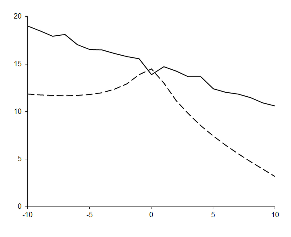
Figure 7 shows the actual (solid line) and estimated (dashed line) decimal digits of accuracy in the approximate derivative of the exponential function using our implementation of Ridders’ algorithm.
|
| Figure 7 |
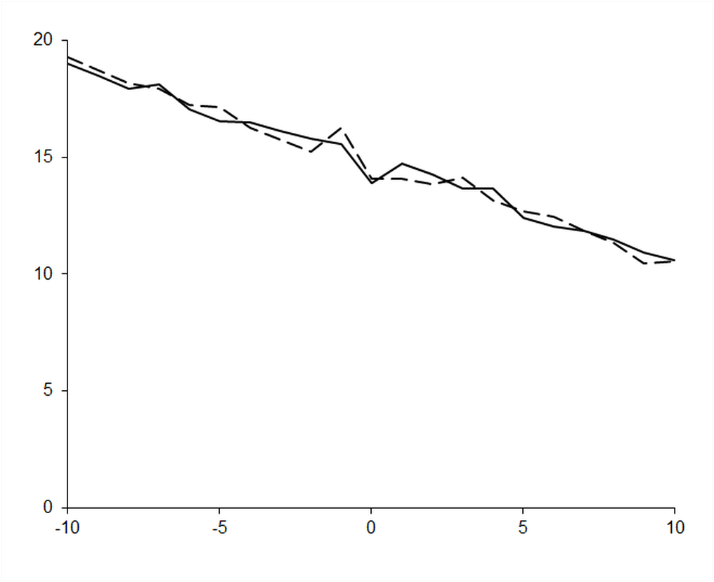
This represents a vast improvement in both accuracy and error estimation over every algorithm we have studied thus far. Figure 8 demonstrates the former with a comparison of the results of Ridders’ algorithm (solid line) and a 7 0 order polynomial approximation (dashed line) using the improved version of our original algorithm based on the truncated Taylor series.
|
| Figure 8 |
The relative error in these results is on average roughly 2E-15, just one decimal order of magnitude worse than the theoretical minimum.
We have thus very nearly escaped the clutches of numerical error and I therefore declare polynomial approximation of the derivative, in this its final and most effective form, a giant amongst ducks; QUAAAACK!
References and further reading
[Press92] Press, W.H. et al, Numerical Recipes in C (2nd ed.), Cambridge University Press, 1992.
[Ridders82] Ridders, C.J.F., Advances in Engineering Software , Volume 4, Number 2., Elsevier, 1982.