We now know that floating point arithmetic is the best we can do. Richard Harris goes back to school ready to show how to use it.
We have travelled far and wide in the fair land of computer number representation and have seen the unmistakable scorch marks that betray the presence of the dragon of numerical error. No matter where we travel we are forced to keep our wits about us if we fear his fiery wrath.
Those who take sport in the forests of IEEE 754 floating point arithmetic have long since learnt when and how the dragon may be tamed and, if we seek to perform mathematical computation, we would be wise to take their counsel.
In this second half of this series of articles we shall take it as read that floating point arithmetic is our most effective weapon for such computation and we shall learn that, if we wish to wield it effectively, we are going to have to think!
To illustrate the development and analysis of algorithms for mathematical computation we shall continue to use the example of numerical differentiation with which we seek to approximate as accurately as possible the derivative of a function, primarily because it is the simplest non-trivial numerical calculation that I know of.
Before we do so, it will be useful to discuss exactly what we mean by differentiation and the tools that we shall exploit in the development and analysis of our algorithms.
On the differential calculus
The aim of the differential calculus is the calculation of the instantaneous rate of change of functions or, equivalently, the slopes of their graphs at any given point.
Credit for its discovery is often given to the 17th century mathematicians Newton and Leibniz, despite the fact that many of the concepts were discovered centuries before by the Greeks, the Indians and the Persians. That said, the contributions of Newton and Leibniz were not insignificant and it is their notations that are still used today:
 from Newton and
dy
/
dx
from Leibniz.
from Newton and
dy
/
dx
from Leibniz.
The central idea of the differential calculus was that of the infinitesimals; hypothetical entities that have a smaller absolute value than any real number other than zero.
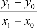
To see how infinitesimals are used to calculate the slope of a graph, first consider the slope of a straight line connecting two points on it, say ( x 0 , y 0 ) and ( x 1 , y 1 )
To compute its slope at a point x we should ideally want to set both x 0 and x 1 equal to x but unfortunately this yields the meaningless quantity 0/0.
Instead we shall set x 0 equal to x and x 1 equal to x plus some infinitesimal quantity dx . Since this is closer to x than any real number, it should yield a result closer to the slope at x than any real number. The actual slope can therefore be recovered by discarding any infinitesimals in that result.
For example, consider the slope of the function x 2 .
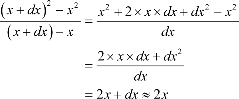
where the wavy equals sign means approximately equal to in the sense that no real number is closer to the result.
We define a function to be continuous if an infinitesimal change in its argument yields an infinitesimal change of the same or higher order in its value. If the same can be said of its derivative, we say that the function is smooth.
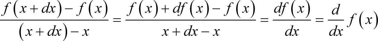
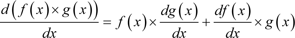
For a smooth function f we therefore have f ( x + dx )= f ( x )+ df ( x ), where df ( x ) is an infinitesimal of at least the same order as dx . Given this we can obtain Leibniz’ notation
That we require the function to be smooth rather than simply continuous might come as a bit of a surprise, but stems from the fact that a function does not have a well defined value at a discontinuity.
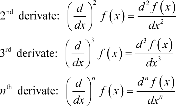
Treating d / dx as an operator as above, we recover the notation for repeated differentiation. We square it if we differentiate twice, cube it if thrice, and so forth, to obtain
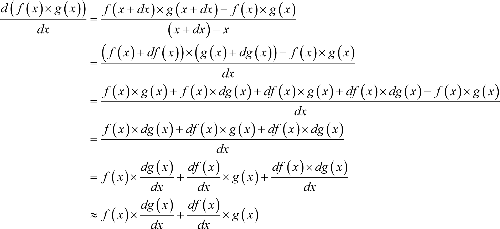
We can recover the various identities of the differential calculus using infinitesimals. In derivation 1, for example, we prove the product rule for the derivative of the product of two functions f and g .
|
Proving the product rule with infinitesimals Given smooth continuous functions f and g :
|
| Derivation 1 |
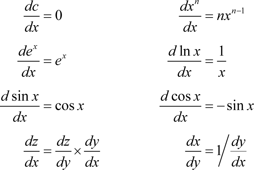
Given constant c , the exponential function e x , its inverse ln x and functions f and g such that y = f ( x ) and z = g ( y ) some further useful identities are
Whilst infinitesimals provide a reasonably intuitive framework for the differential calculus it is not a particularly rigorous one. What exactly does it mean to say that an infinitesimal is smaller in magnitude than any real number other than zero? Given any real number, we can halve it to give us a number that is closer to zero. Halving again yields a number closer still, as does halving a third time. Repeating this process over and over again yields a sequence of numbers that shrink arbitrarily close to zero, so where exactly are the infinitesimals to be found?
This lack of rigour did not escape Newton and Leibniz’ contemporaries; the philosopher George Berkeley [ Berkeley34 ], for example, criticised the calculus for its ‘ fallacious way of proceeding to a certain Point on the Supposition of an Increment, and then at once shifting your Supposition to that of no Increment ’ and derided the infinitesimals as the ‘ ghosts of departed quantities ’.
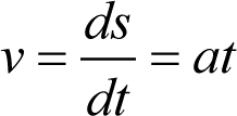
Despite these objections, many mathematicians were unwilling to dismiss the differential calculus due to its incredible usefulness. For example, consider the equation governing the straight line distance s travelled in a time t by a frictionless body from a standing start under a constant acceleration a
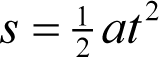
If we take the derivative of this with respect to time, we recover the equation governing the speed of that body after the time t
That equations of motion such as these could be experimentally verified was rather strong evidence that the differential calculus was valid. It was not until some 150 years later that this was conclusively demonstrated, however.
On analysis
It was Cauchy who made the great leap forward in setting the differential calculus on a secure foundation. He did it not by giving the infinitesimals a rigorous definition but by doing away with them entirely.
His idea was to define the derivative as the limit of a sequence of ever more accurate approximations to it. Specifically, that
is the limit of
as Δ x tends to 0
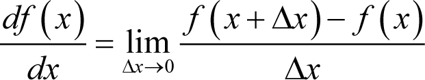
or in conventional notation
For example, consider again the derivative of x 2
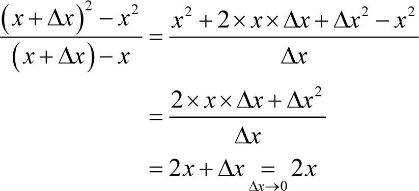
where the final equals sign means equals as Δ x tends to zero .
Now this is how we defined the derivative in the first article in this series but, whilst it’s certainly a step in the right direction, it’s not yet quite enough. What exactly do we mean when we say Δ x tends to zero? Do we repeatedly halve it? Do we start with a positive value less than 1 and square it, then cube it, then raise it to the 4th power and so on? Does it actually matter ?
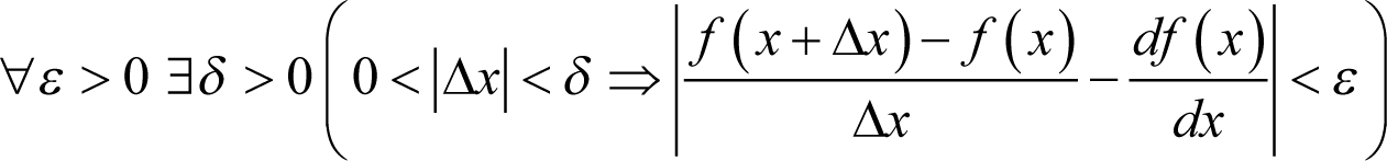
Cauchy’s great achievement was to rigorously define the limit of a sequence and, in doing so, discover analysis: the mathematics of limits. We say that the limit of a function f ( x ) as x tends to c is equal to l if and only if for any given positive ε, no matter how small, we can find a positive δ such that the absolute difference between f ( x ) and l is always less than ε if the absolute difference between x and c is less than δ . In mathematical notation we write this as

where the upside down A should be read as for all , the backwards E as there exists , and the arrow as implies that . The vertical bars represent the absolute value of the expressions bracketed by them.
With this definition we are not dependant upon the manner in which we approach a limit, only upon the size of its terms.
We now define the derivative df ( x )/ dx with
If such a limit exists, we say that the function is differentiable at x .
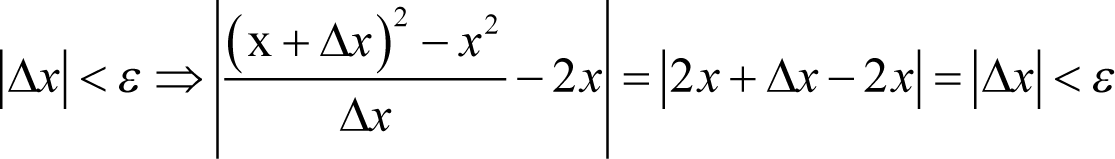
The derivative of x 2 is 2 x since for all x
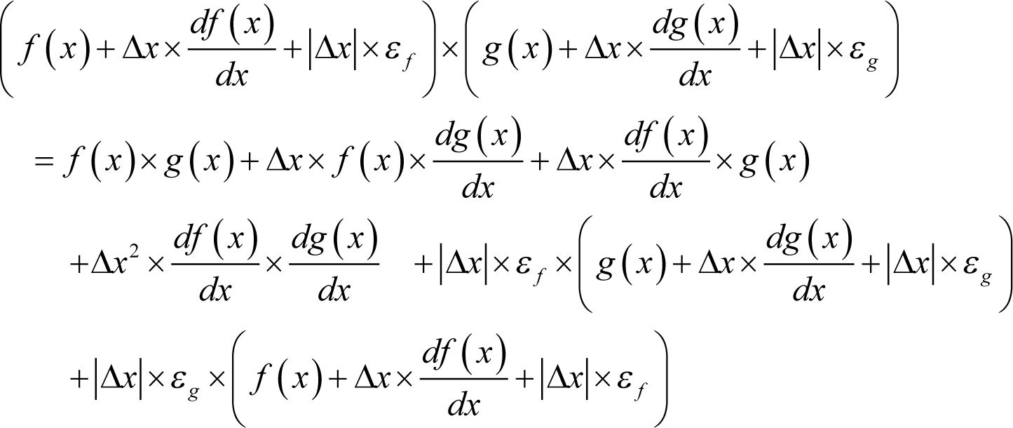
As we did with infinitesimals, we can derive the various identities of the differential calculus with this rigorous definition of a limit. Derivation 2 provides a proof of the product rule in these terms, for example.
|
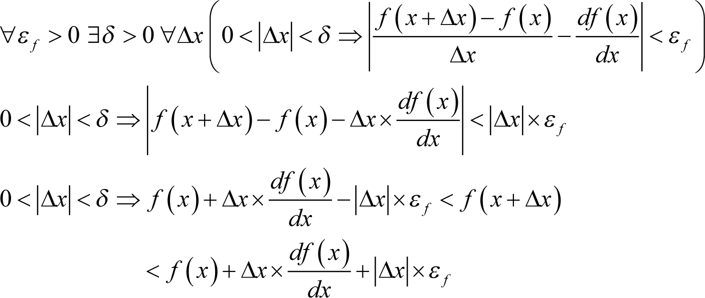
Proving the product rule with limits Given a differentiable function f we have
Now, given a second differentiable function g we have
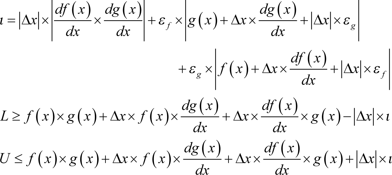
The bounds on the product of f ( x +Δ x ) and g ( x +Δ x ) are the minimum and maximum of the four possible products of their bounds of which, if we denote them by L and U , we can be sure that
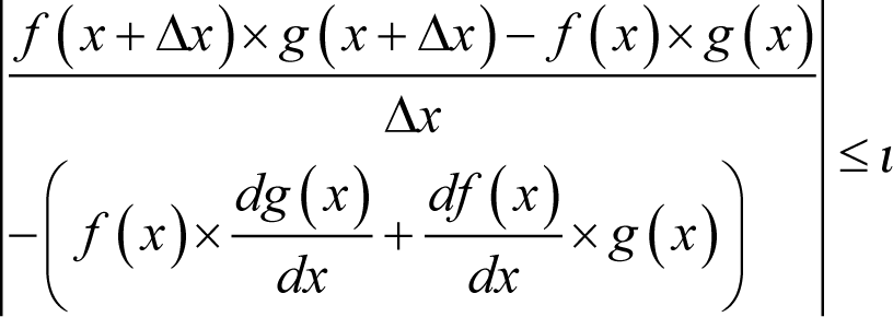
and hence that
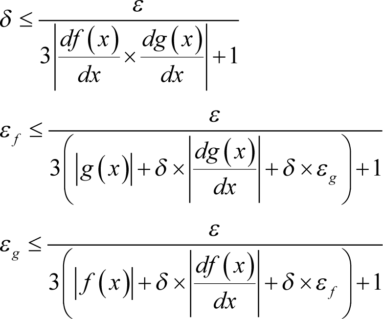
For any given positive ε we can, for example, choose positive δ such that
and thus i < ε whenever |Δ x |< δ , as required. |
| Derivation 2 |
That this proof is so much longer and more difficult than the one using infinitesimals is something that mathematicians have had to learn to live with; the price of rigour is generally paid in ink. The rigour that Cauchy brought to the differential calculus was part of a great revolution in mathematical thinking that took place during the 19th century. Indeed, almost all of the techniques of modern mathematics were developed during this period.
Infinitesimals two point 0
In the latter half of the 20th century the infinitesimals enjoyed something of a renaissance. Both Robinson, with his non-standard numbers [ Robinson74 ], and Conway, with his surreal numbers [ Knuth74 ], developed consistent number systems in which infinitesimals could be given a rigorous definition.
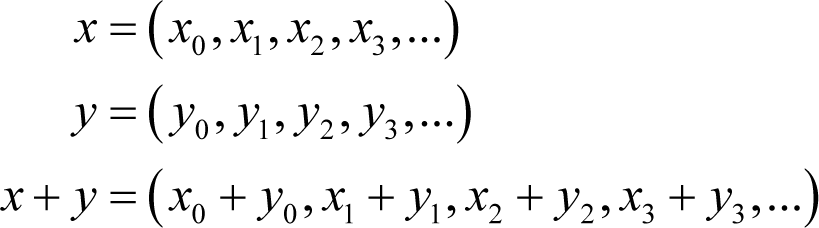
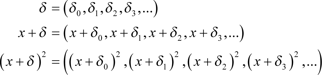
Their approach was to embed something akin to Cauchy’s limits into the very idea of a number. Loosely speaking, Robinson defined a non-standard number as an infinite sequence of real numbers with arithmetic operations and functions applied on an element by element basis. For example
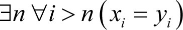
Loosely speaking, two non-standard numbers x and y are considered equal if for all but a finite set of indices i , x i = y i or, in limit notation, that
The remaining comparison operators are similarly defined and the real numbers are the subset of the non-standard numbers whose elements are identical for all but a finite set of indices. Now consider the standard number whose elements are a strictly decreasing sequence of positive numbers. For example
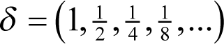
By the rules of non-standard arithmetic this number is greater than zero since every element in it is greater than zero. Furthermore, it is smaller than any positive real number x since there will be some n for which 1/2 n is smaller than x and hence so will be the infinite sequence of elements of δ after the n th . So here we have a genuine, bona fide infinitesimal with all of the properties of those in Newton and Leibniz’ differential calculus!
If a non-standard number z can be represented by a real number plus an infinitesimal non-standard number, we call that real number the standard part of z , or st( z ). We can thus define the derivative of a function f as
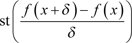
for a standard real x and all infinitesimal non-standard δ , if this value exists. For example, let’s consider the derivative of x 2 a third time.
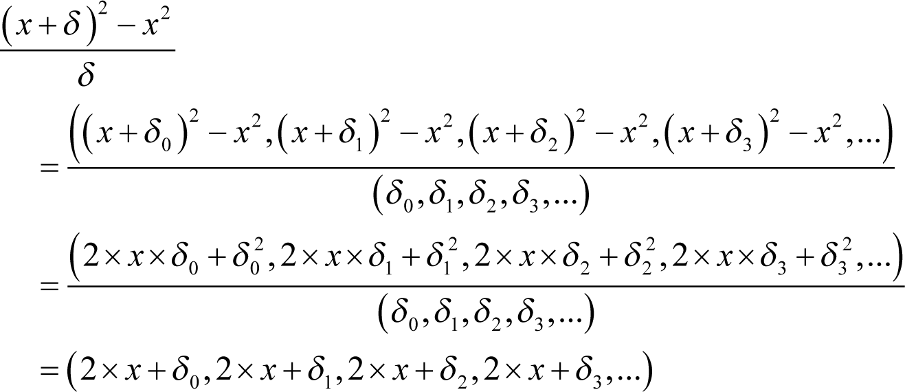

Note that at no point did we rely upon the value of δ , just that it was an infinitesimal, and hence the result stands for all infinitesimals.
The problem with this loose definition of the non-standard numbers is that the vast majority of them are comprised of oscillating or random sequences which cannot meaningfully be ordered by the less than and greater than operators. Fortunately, the formal definition addresses this deficiency by demonstrating that it is possible to define rules by which we can do so, albeit ones which we cannot ever hope to write down in full.
Very roughly speaking, these rules unambiguously equate oscillating/ random sequences with convergent or divergent sequences. By magic.
Robinson proved that the non-standard numbers do not lead to any logical contradictions other than those, if any, that are consequences of the standard reals and that his infinitesimals have exactly the properties of Newton’s.
We can therefore dispense with the full limit notation and simply go back to using our original infinitesimals.
Now that we know exactly how the differential calculus is defined we are nearly ready to begin analysing numerical differentiation algorithms.
Before we can start, however, there is one last piece of mathematics that we shall need.
Taylor’s theorem
For those who seek to develop numerical algorithms, Taylor’s theorem is perhaps the single most useful result in mathematics.
It demonstrates how a sufficiently differentiable function can be approximated within some region to within some error by a polynomial. Specifically, it shows that
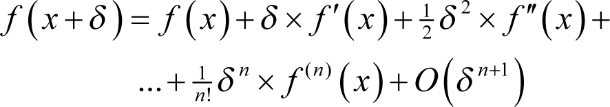
where we are using the notational convention of f' ( x ) for the derivative of f evaluated at x , f" ( x ) for the second derivative and f ( n ) ( x ) for the n th derivative. The exclamation mark is the factorial of, or the product of every integer from 1 up to and including, the value preceding it. O ( δ n +1 ) is an error term of order δ n +1 or, in other words, that for any given f and x is equal to some constant multiple of δ n +1 .
By sufficiently differentiable we mean that all of the derivatives of f up to the n +1 th must exist, and that all of the derivatives of f up to the n th must be continuous, between x and x + δ , inclusive of the bounds in the latter case but not in the former.
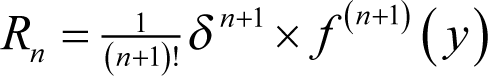
In fact, the error term has exact bounds given by a more accurate statement of Taylor’s theorem
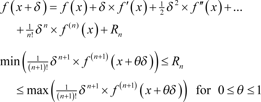
or, equivalently, that for some y between x and x + dx
If we put no limit upon n we recover the Taylor series of a function f in the region of x
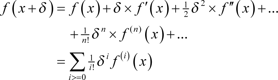
where the capital sigma stands for the sum of the expression to its right for every unique value of i that satisfies the inequality beneath it and with the factorial of 0 being 1 and the 0 th derivative of a function being the function itself. Note that this identity holds if and only if the sum has a well defined limit under Cauchy’s definition.
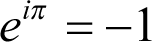
We can use Taylor series about 0, also known as Maclaurin series, to prove the surprising relationship between the value of the exponential function at 1, e , the ratio of the circumference of a circle to its diameter, π, the square root of -1, i , and -1
We do this by examining the Maclaurin series of the exponential function, the sine function and the cosine function
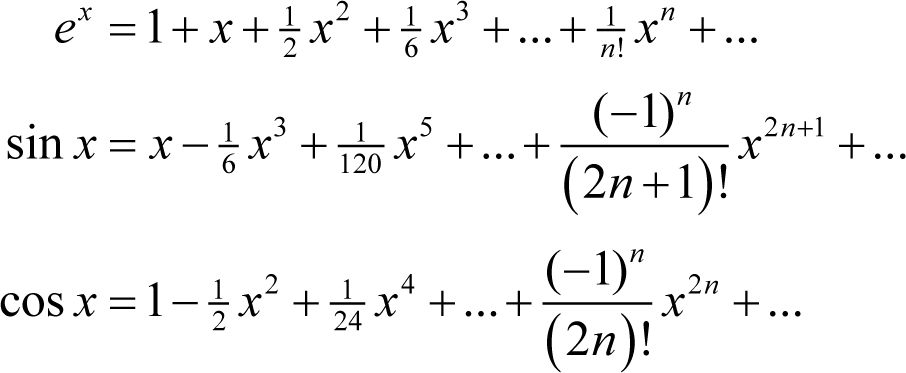
Note that all three of these series converge for any value of x and can be extended to the complex numbers that are the sums of real numbers and multiples of i .
So let’s now consider e ix
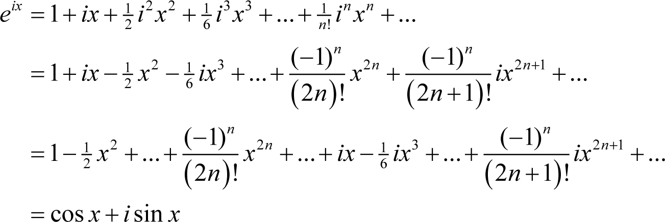
This is known as Euler’s formula and yields that surprising relationship when we set x =π.
As fascinating and profound as this undoubtedly is, it is not the reason that Taylor’s theorem is of such utility in numerical computing. Rather, it is that Taylor’s theorem provides us with an explicit formula for approximating a function with a polynomial and bounds on the error that results from doing so.
Such polynomials are very easy to mathematically and numerically manipulate and thus can dramatically simplify many mathematical computations; they are used to very great effect in Physics, for example.
Furthermore, it gives us an explicit formula for the error in the value of a function that results from an error in its argument, such as might occur through floating point rounding for example
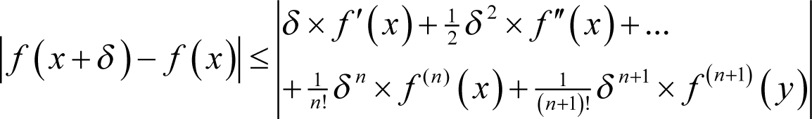
for some y between x and x + δ that maximises the right hand side of the equation.
So, now we have a thorough grasp of the differential calculus and are equipped with the numerical power tool of Taylor’s theorem, we are ready to scrutinise some of the numerical algorithms for approximating the derivatives of functions.
I’m afraid we shall have to wait until next time before we do so, however.
References and further reading
[Berkeley34] Berkeley, G., The Analyst; Or, A Discourse Addressed to an Infidel Mathematician , Printed for J. Tonson, 1734.
[Knuth74] Knuth, D., Surreal Numbers; How Two Ex-Students Turned on to Pure Mathematics and Found Total Happiness , Addison-Wesley, 1974.
[Robinson74] Robinson, A., Non-Standard Analysis , Elsevier, 1974.