We now have the tools to analyse the Countdown Numbers Game. Richard Harris is ready to play.
In the first part of this article we described the numbers game from that Methuselah of TV quiz shows, Countdown [ Countdown ]. The rules of this game are that one of a pair of contestants chooses 6 numbers from a set of 4 large numbers and another of 20 small numbers, comprised respectively of the integers 25, 50, 75 and 100 and 2 of each of the integers from 1 to 10.
Over the course of 30 seconds both contestants attempt to discover a formula using the 4 arithmetic operations of addition, subtraction, multiplication and division and, no more than once, each of the 6 integers that results in a randomly generated target between 1 and 999 that has no non-integer intermediate values.
Reverse Polish Notation
Since we shall need to automatically generate formulae during any statistical analysis of the property of this game, we introduced Reverse Polish Notation, or RPN. Supremely well suited to computational processing, RPN places operators after the arguments to which they are applied, rather than between them as does the more familiar infix notation.
RPN utilises a stack to keep track of intermediate values during the processing of a formula and in doing so removes the need for parentheses to determine the order in which operators should be applied. Whenever a number appears in the input sequence it is pushed on to the stack and whenever an operator appears it pops its arguments off of the stack and pushes its result back on to it.
Formula templates
To simplify the enumeration of the set of possible formula, we introduced formula templates in which arguments are represented by x symbols and operators by o symbols. We described a scheme for recursively generating every possible formula template for up to a given number of arguments by repeatedly replacing x symbols with the sequence of symbols xxo .
The declaration of our C++ implementation of this scheme (the all_templates function) is:
      std::set<std::string> all_templates(
         size_t arguments);
We concluded the first part of this article by implementing a mechanism with which we could evaluate formula template for a given set of operators and arguments.
We began by implementing an abstract base class to represent arbitrary RPN operators for a given type of argument, as illustrated in listing 1 together with the declarations of the 4 operator classes that are derived from it.
template<class T>
    class rpn_operator
    {
    public:
      typedef
         std::stack<std::vector<T> >  stack_type;
      virtual ~rpn_operator();
      virtual bool apply(stack_type &stack) const = 0;
    };
    template<class T> class rpn_add;
    template<class T> class rpn_subtract;
    template<class T> class rpn_multiply;
    template<class T> class rpn_divide;
|
| Listing 1 |
Note that the return value of the apply member function indicates whether the result of the calculation has a valid value.
The implementation of the rpn_divide class is illustrated in listing 2. The remaining operators are implemented in much the same way, although divide is the only one that needs to check the validity, rather than just the availability, of its arguments and can therefore return false from its apply method. Specifically, it requires that for double arguments the second must not be equal to 0 and that for long arguments it must also wholly divide the first.
template<class T>
    class rpn_divide : public rpn_operator<T>
    {
    public:
      virtual bool apply(stack_type &stack) const;
    };
|
| Listing 2 |
Note that the operator classes themselves are responsible for checking that the correct number of arguments are available, since this allows us to implement operators taking any number of arguments, should we so desire.
We then implemented the rpn_result structure to represent both the validity and the value of the result of a formula, as illustrated in listing 3.
template<class T>
    struct rpn_result
    {
      rpn_result();
      explicit rpn_result(const T &t);
      bool valid;
      T    value;
    };
|
| Listing 3 |
Finally, we implemented a function that, given a string representing a formula template, a container of pointers to rpn_operator base classes and a container of arguments, yields the result of the formula generated by substituting the operators and arguments in sequence into the template. We plumped for the rather unimaginative name, rpn_evaluate , whose declaration is illustrated in listing 4.
template<class T>
    rpn_result<T>
    rpn_evaluate(const std::string &formula,
                 const std::vector<rpn_operator<T>
                 const *> &operators,
                 const std::vector<T> &arguments);
|
| Listing 4 |
Evaluating every formula for a given template
To examine the results of every possible formula in the Countdown numbers game we shall need to call the rpn_evaluate function for every one of the templates we have for up to 6 arguments with every possible set of operators and arguments. Recalling the formula we deduced for the total number of possible formulae

we concluded that we would need a mechanism of enumerating, for each n argument template, the 4 n -1 choices of operators and the 6 P n permutations of arguments in addition to a mechanism for enumerating the 24 C 6 combinations of 6 from the 24 available numbers.
You will no doubt recall that a permutation is the number of ways we can select a subset of elements from a set when order is important and that a combination is the number of ways that we can select such a subset when order isn't important.
In the second part of this article we sought these mechanisms.
Fortunately for us, we created the first of them during our study of knots [ Harris08 ]. The declaration of the next_state function that enumerates every possible state of a collection of integer-like objects is given below:
      template<class BidIt, class T>
      bool
      next_stateFidIt first, BidIt last, const T &ub,
         const T &lb = T());
Since the next_state function is only applicable to iterator ranges of integer-like objects, we shall ultimately need to place our 4 operators in a container and use this function in conjunction with iterators ranging over it.
Generating the set of permutations was a little more complicated since the standard next_permutation function does not generate permutations of subsets. Fortunately, however, we were able to exploit the fact that it generates full sets of permutations in lexicographical order to trick it into generating permutations of subsets for us by reverse sorting the elements from mid to last . Our next_permutation function enumerated the set of permutations of mid - first from last - first items in lexicographical order.
      template<class BidIt>
      bool
      next_permutation(BidIt first, BidIt mid,
         BidIt last);
We then, rather tediously I suspect, devised our own algorithm for enumerating combinations in lexicographical order and finally, slightly less tediously I hope, implementing it. The declaration of the next_combination function in which we implemented our algorithm is provided below.
      template<class BidIt>
      bool
      next_combination(BidIt first, BidIt mid,
                       BidIt last);
Putting it all together again
We concluded by implementing a function to iterate over every possible numbers game and pass their results to a statistics gathering function. We first needed some functions to convert between the sequences of values and iterators that our rpn_evaluate and argument and operator choice enumeration functions expected, as declared in listing 5.
template<class FwdIt> void
    fill_iterator_vector(FwdIt first, FwdIt last,
                         std::vector<FwdIt> &vec);

    template<class FwdIt, class T>
    void
    fill_dereference_vector(FwdIt first, FwdIt last,
                            std::vector<T> &vec);
|
| Listing 5 |
We built the function to enumerate the possible games in two parts, the first of which iterated through the combinations of selections of numbers to work with, and the second of which iterated through every possible game that can be played with those numbers. The declarations of these two functions are illustrated in listing 6.
template<class BidIt, class Fun>
    Fun
    for_each_numbers_game(BidIt first, BidIt last,
       size_t args, Fun f);
    template<class BidIt, class Fun>
    Fun
    for_each_numbers_game(BidIt first_number_choice,
       BidIt last_number_choice, Fun f);
|
| Listing 6 |
We concluded that we were finally ready to begin analysing number games and we are indeed ready to do so.
Counting the number of valid games
Since the Countdown numbers game does not allow fractions, our formula for counting the number of formulae is going to overestimate the total number of valid games. I'm reasonably confident that I won't be able to derive an explicit formula to take this into account, so propose instead that we count them using our for_each_numbers_game functions.
Recall that our calculation implied that the number of formulae that could be constructed from 6 arguments chosen from 24 numbers was equal to 4,531,228,985,976, somewhat larger than can be represented by a 32 bit unsigned integer. We shall therefore recruit our accumulator class from our analysis of prime factorisations of integers [ Harris09 ], given again in listing 7
class accumulator
    {
    public:
      accumulator();
      accumulator & operator+=(unsigned long n);
      operator double() const;

    private:
      std::vector<unsigned long> n_;
    };

    accumulator::accumulator() : sum_(1, 0)
    {
    }

    accumulator &
    accumulator::operator+=(unsigned long n)
    {
      assert(!sum_.empty());
      sum_.front() += n;
      if(sum_.front()<n)
      {
        std::vector<unsigned long>::iterator first =
           sum_.begin();
        std::vector<unsigned long>::iterator last  =
           sum_.end();
        while(++first!=last && ++*first==0);
        if(first==last)  sum_.push_back(1);
      }
      return *this;
    }
|
| Listing 7 |
To check whether the result of an in-place addition requires additional storage we exploit the fact that in C++ unsigned integers don't overflow, but that it instead treats arithmetic using n bit unsigned integers as being modulo 2 n [ ANSI98 ].
We use the accumulator class in a function object that counts the number of valid formulae by adding 1 to the count every time it is called with the result of a calculation, as shown in listing 8.
class
    count_valid
    {
    public:
      void operator()(long);
      const accumulator & count() const;

    private:
      accumulator count_;
    };

    void
    count_valid::operator()(long)
    {
      count_ += 1;
    }

    const accumulator &
    count_valid::count() const
    {
      return count_;
    }
|
| Listing 8 |
Unfortunately, a preliminary investigation suggested that the calculation of the total number of valid games would take the best part of 2 months of CPU time using the admittedly rather outdated PC upon which I am writing this essay.
Turbo-charging the stack
We can improve matters somewhat by abandoning the standard stack and implementing our own. This will exploit the short string optimisation to keep the bottom of the stack on the much faster local store. If your STL implementation already uses the short string optimisation for its vector s, then this won't really make much difference. Mine doesn't, so it will offer me an advantage, at least. The declaration of this class is given in listing 9.
template<class T, size_t N,
       class Cont=std::deque<T> >
    class rpn_stack
    {
    public:
      typedef T      value_type;
      typedef size_t size_type;

      rpn_stack();

      bool      empty() const;
      size_type size() const;

      const value_type & top() const;
      void push(const value_type& x);
      void pop();

    private:
      rpn_stack(const rpn_stack &other);
      //not implemented
      rpn_stack & operator=( const rpn_stack &other);
      //not implemented

      std::stack<T, Cont> overflow_;
      value_type          data_[N];
      value_type *        top_;
    };
|
| Listing 9 |
Note that this isn't intended as a drop in replacement for the standard stack , since it only implements the member functions we require for an RPN calculation.
We use the trick of privately declaring, but not defining, the copy constructor and assignment operator to suppress the compiler generated defaults and ensure than an error will result if we accidentally use them. We don't ever need to copy stack objects during the evaluation of an RPN formula, and the defaults would leave them with pointers into each other's member arrays.
We include a standard stack to cope with values that drop off the end of our member array. The implementation of the member functions is fairly straightforward, as illustrated in listing 10.
template<class T, size_t N, class Cont>
    rpn_stack<T, N, Cont>::rpn_stack() : top_(data_)
    {
    }

    template<class T, size_t N, class Cont>
    bool
    rpn_stack<T, N, Cont>::empty() const
    {
      return top_==data_;
    }

    template<class T, size_t N, class Cont>
    rpn_stack<T, N, Cont>::size_type
    rpn_stack<T, N, Cont>::size() const
    {
      return (top_-data_) + overflow_.size();
    }

    template<class T, size_t N, class Cont>
    const rpn_stack<T, N, Cont>::value_type &
    rpn_stack<T, N, Cont>::top() const
    {
      return overflow_.empty() ? *(top_-1) :
         overflow_.top();
    }

    template<class T, size_t N, class Cont>
    void
    rpn_stack<T, N, Cont>::push(const value_type &x)
    {
      if(top_!=data_+N)  *top_++ = x;
      else               overflow_.push(x);
    }

    template<class T, size_t N, class Cont>
    void
    rpn_stack<T, N, Cont>::pop()
    {
      if(overflow_.empty())  --top_;
      else                   overflow_.pop();
    }
|
| Listing 10 |
We are using the data_ member array to store the first N values on the stack and so initialise the top_ pointer to the start of it during construction. It shall always point to the element immediately following the last value on the stack that is stored in the member array. Only when we have exhausted the array will we use overflow_ .
The empty member function therefore simply compares the top_ pointer to the start of the member array.
Similarly, the size member function simply adds the number of values we currently have in our member array to the size of overflow_ . If the former is full, the top_ pointer will be equal to data_+N and so size will correctly return the size of overflow_ plus N . If not, the latter will be empty and size will return the number of values currently in the member array.
The top member function defers to overflow_ if it is not empty, otherwise returns the value immediately before top_ . Note that, like the standard stack , we do not check that there are any values currently on the stack.
The push member function assigns the pushed value to the element pointed to by top_ and increments top_ if it is not already at the end of the member array. If it is, the function simply defers to overflow_ .
Similarly, if overflow_ is empty, the pop member function simply decrements top_ . If it is not, the function defers to it instead. Note that this function, like top , does not perform any check that there are any values currently on the stack.
Finally, we should note that since the values stored in the member array are not destroyed until the rpn_stack is, it is not particularly useful for values that consume lots of resources.
Listing 11 shows the change that we need to make to the rpn_operator class to use the rpn_stack . Note that I'm only putting the first 6 values on the stack in local storage since during our analysis of the Countdown numbers game this will be the maximum number of arguments we shall use. Whilst this is clearly not a generally justifiable choice, I suspect that we'd be hard pushed to find another application for which we would really care quite this much about RPN formula calculation efficiency, so I figure it's probably OK.
template<class T>
    class rpn_operator
    {
    public:
      typedef rpn_stack<T, 6>  stack_type;
      ...
    };
|
| Listing 11 |
Using our new stack brings the calculation time for counting every valid formula down to a little under 3 weeks. A fair bit better to be sure, but still not exactly tractable.
Whilst I'm sure that we could find a yet more efficient approach with a little more work, I rather suspect that it wouldn't consist of such satisfyingly independent constructs. That said, if there's some blindingly obvious improvement that doesn't muddle up the responsibilities of our various functions and classes, I'd be more than happy to hear about it.
The Countdown numbers game's little brothers
To keep the calculation manageable, I therefore suggest that we instead consider a cut down version of the numbers game; one in which we choose our 6 arguments from the set of 4 large numbers and half of the set of small numbers, or in other words 1 of each of the integers from 1 to 10.
Another back of the envelope calculation suggests that this should take approximately 10 hours; hardly nippy, but not completely out of the question.
Multiplying the number of formulae we can construct with up to 6 arguments by the number of ways in which we can select 6 arguments from 14 without taking order into account, or 14 C 6 , yields a total of 101,097,214,218 possible formulae, still a smidge out of the range of a 32 bit unsigned integer.
The result of our calculation for this smaller numbers game shows that there are just 32,215,124,261 valid formulae, less than a third of the total number of formulae. The 68,882,089,957 invalid formulae must all involve division since that's the only operator that can have an invalid result. We can easily count the number of formulae involving division operations by subtracting from our total the number of formulae that involve only addition, subtraction and multiplication (we calculate this by replacing the 4 with a 3 in our formula). Doing so indicates that there are exactly 76,425,599,250 formulae involving division, of which over 90% are invalid.
This leads me to wonder what might happen to the ratio between valid integer-only formulae and total formulae as we increase the number of arguments. This calculation will be more expensive still, so we shall examine games using 1 of each of the integers from 1 to 8 with from 1 to 8 arguments. The results of this calculation are given in figure 1.
| The proportion of valid formulae of all formulae and formulae involving division |

|
| Figure 1 |
As fascinating as this almost is, it's high time we got around to investigating the statistical properties of the game. Specifically, I should like to know what the distribution of the results of every valid numbers game looks like.
Building a histogram of numbers game results
Since the results of the numbers game formulae are integers, their distribution will be discrete and hence naturally represented with a histogram. Listing 12 provides the declaration of the histogram class we shall use.
class game_histogram
    {
    public:
      game_histogram();
      game_histogram(long lower_bound,
                     long upper_bound);

      long   lower_bound() const;
      long   upper_bound() const;
      double samples() const;

      double operator[](long i) const;
      void   operator()(long i);

    private:
      typedef accumulator             value_type;
      typedef std::vector<value_type> histogram_type;

      long           lower_bound_;
      value_type     samples_;
      histogram_type histogram_;
    };
|
| Listing 12 |
It is a little less fully featured than the histograms we have implemented for previous studies, although since it uses our accumulator class to keep count of the samples it can deal with much larger numbers.
We can afford a reduced interface since the sample values will be integers and will thus serve perfectly well as indices into the histogram. Note that the function call operator overload is used to add samples since this enables us to use the game_histogram class as the function object expected by our for_each_numbers_game function.
Listing 13 illustrates the definitions of the member functions. These are reasonably straightforward, with the only real gotcha being that the lower_bound and upper_bound are inclusive bounds of the histogram.
    game_histogram::game_histogram() : lower_bound_(0)
    {
    }

    game_histogram::game_histogram(long lower_bound,
                                   long upper_bound) :
             lower_bound_(std::min(lower_bound,
                                   upper_bound)),
             histogram_(size_t(labs(
                        upper_bound-lower_bound)+1))
    {
    }

    long
    game_histogram::lower_bound() const
    {
      return lower_bound_;
    }

    long
    game_histogram::upper_bound() const
    {
      return lower_bound_ + (
         long(histogram_.size()) - 1);
    }

    double
    game_histogram::samples() const
    {
      return samples_;
    }

    double
    game_histogram::operator[](long i) const
    {
      if(i<lower_bound() || i>upper_bound())
         return 0.0;
      return histogram_[size_t(i-lower_bound_)];
    }

    void
    game_histogram::operator()(long i)
    {
      samples_ += 1;
      if(i>=lower_bound() && i<=upper_bound())
      {
        histogram_[size_t(i-lower_bound_)] += 1;
      }
    }
|
| Listing 13 |
When trying to read values outside of the stored range we simply return 0, and when trying to add them the histogram entry is quietly dropped and only the count of the number of samples is increased.
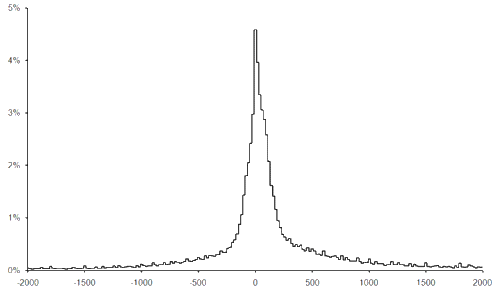
The histogram generated with this class enumerated over every game with the 4 large numbers and the 10 small numbers with results ranging from -2000 to +2000, grouped into buckets of 20 results to smooth out the graph a little, is shown in figure 2.
|
| Figure 2 |
There are clearly more positive results than negative, which should be expected since we can only generate a negative result by subtracting some formula from 1 of the 6 selected numbers, leaving that formula with only 5 or fewer arguments.
It is worth noting that the formulae with results in the range of our histogram account for just a little over 70% of the valid games.
I must admit that I'm a little surprised by the shape of the histogram. I was expecting it to look like a discretisation of the normal distribution since that, as you will remember from our previous studies, is the statistical distribution of sums of random numbers.
Any formula can be recast as a sum of terms involving just multiplication and division by expanding out any terms in brackets, something known as the distributive law of arithmetic. For example, we can expand the formula
a × ( b + c )
into
( a × b ) + ( a × c )
With an admittedly rather hand-waving argument I had imagined that these terms could be thought of as random variables in their own right. Whilst the terms would clearly not be independent in general, I believed that assuming that they were would yield a reasonable approximation.
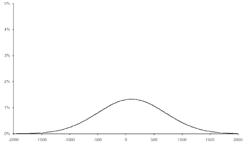
The average, or mean, of our truncated histogram is approximately 100, whilst its standard deviation (the square root of the average squared difference from the mean) is approximately 600. The histogram that would result from a normal distribution with these parameters is shown in figure 3 for comparison with our histogram of numbers game results.
|
| Figure 3 |
Clearly I was very much mistaken.
So what kind of distribution do the results of the numbers games exhibit?
The histogram of the absolute values of numbers game results
In pursuit of a statistical distribution that might describe the numbers game, I suggest that we allow the result of a formula to be negated. There are trivially twice as many formulae that can be constructed and the distribution of the results must be symmetric about 0. We can therefore simply study the histogram of the absolute results (i.e. ignoring the sign) which we can build by adding together the histogram value for each positive result to the value for its negation, and from which we can easily construct the full distribution.
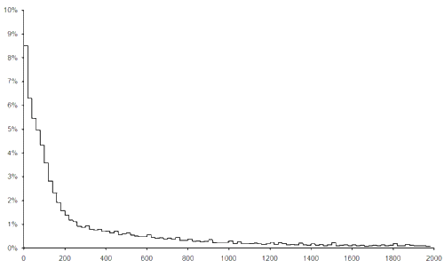
Figure 4 illustrates the histogram of the absolute results, also constructed with buckets of 20 results.
|
| Figure 4 |
The fact that this distribution falls away to 0 so slowly is highly suggestive of the class of distributions it falls into; the power law distributions.
Power law distributions
Power law distributions have the probability density functions of the form

where L is a slowly varying function, or in other words has the limiting behaviour

for constant t [ Clauset09 ]. The lim term on the left hand side of the fraction stands for the limit as x grows ever larger of the term to its right. We can interpret the equation as meaning that the function L should get closer and closer to a constant as x grows larger and larger.
Probability density functions, or PDFs, are identical to histograms when describing discrete random variables. PDFs are more general, however, in that they can also describe continuous random variables.
Power law distributions are notable because their PDFs decay to 0 very slowly as x increases and are hence associated with processes which display extreme behaviour with surprisingly high probability. The stock market, with its relatively frequent and all too hastily dismissed crashes, is one example that depressingly springs to mind [ Ormerod05 ].
To determine whether a variable has a power law distribution, we can plot the logarithm of its PDF against the logarithm of x . If it follows a power law distribution then for large x this graph will be close to a straight line since
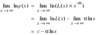
for some constant c .
For sample data, in which there will inevitably be some loss of information, be it noise or gaps in the distribution, we instead sort the n samples in ascending order and, treating the first as having an index of 0, plot ( n - i )/ n against the i th value. This is the discrete equivalent of another test based on the integral of the PDF.
Unfortunately, neither of these tests is particularly accurate. Worse still, accurately determining whether a sample is consistent with a power law distribution is something of an open question with the most reliable current techniques relying upon barrages statistical tests that are far beyond the scope of this article.
Are the absolute numbers games power law distributed?
Our distribution seems to have a lot of little spikes in its tail and furthermore has an upper bound of
100 × 75 × 50 × 25 × 10 × 9 = 843,750,000
beyond which the probability of observing a result is trivially 0. It is therefore certainly not exactly power law distributed, although it is possible that it follows one approximately.
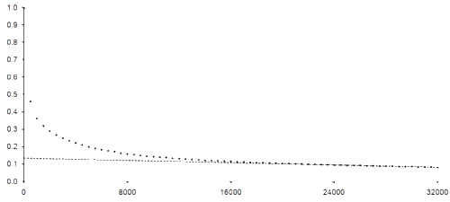
Using the sample data approach of identifying power law behaviour figure 5 plots every 500 th of the sorted results from 0 to 32,000 against the function of their positions in the list together with a straight line drawn through every 500 th of the 24,000 th to the 32,000 th point.
|
| Figure 5 |
Well, it certainly looks very much like a straight line, and with a root mean square error between the line and the points it was drawn through of a little over 0.00025 we can probably conclude that it is at least quite close to one.
Despite this not being a particularly good test for power law behaviour, the cumulative histogram of the numbers game can be approximated for every result in this range by that of a power law with a root mean square error of approximately 0.0003. Statistically speaking, this is actually a fairly significant difference since the histogram is constructed from a huge number of results. Nevertheless, as an approximation it predicts the proportion of results falling below a given value within this range with an error that is everywhere less than a not too shabby 0.061%.
Since we cannot swiftly enumerate every possible formula in the full Countdown numbers game, we shall instead have to randomly sample them if we wish to check whether or not their absolute results are similarly approximated by a power law distribution.
Sampling the Countdown numbers game
To implement a scheme for randomly sampling numbers games, we take similar steps to those we took when implementing a function to enumerate them. Specifically we need a mechanism for the random generation of permutations, of combinations and of operator choices.
Just as our previously implemented next_state function solved the problem of enumerating operator choices, so the random_state function implemented as part of the same article solves the problem of randomly generating them. Implemented in listing 14 together with a random number generator, rnd , it was inspired by the standard random_shuffle function and, like it, does not place many restrictions upon the values on which it operates. This means that we shall not need to use iterators into a container of operators, but will instead be able to use the container directly.
    double
    rnd(double x)
    {
      return x * double(
         rand())/(double(RAND_MAX)+1.0);
    }

    template<class FwdIt, class States>
    void
    random_state(FwdIt first, FwdIt last,
                 const States &states)
    {
      while(first!=last)
      {
        *first++ = states[size_t(
           rnd(double(states.size())))];
      }
    }
|
| Listing 14 |
To generate a random permutation, we can exploit the fact that the standard random_shuffle function has an equal probability of leaving any value in any position. We can therefore simply use it and then just examine the part of the iterator range that we're interested in.
If we then sort that part of the iterator range, we have effectively implemented an algorithm for generating random combinations.
Our scheme shall therefore proceed as follows:
- Pick a formula template at random.
- Pick a set of operators at random.
- Pick a combination of the available numbers at random.
- Pick a permutation of arguments from these at random.
Hang on a sec, those last 2 steps look a bit dodgy to me.
We're picking a sorted random combination of numbers and then an unsorted random permutation of arguments from them. Our algorithms for generating random combinations and permutations require that we apply random_shuffle to the whole range from which each is generated and then ignore those elements we're not interested in. In other words, we shall be sorting the selected numbers to create the combination and then immediately afterwards randomly shuffling them again to generate our permutation of arguments. Isn't this ever so slightly a complete and utter waste of time?
Well, yes it is; we can combine both steps by instead generating a random permutation of the arguments we require from the full set of available numbers:
- Pick a formula template at random.
- Pick a set of operators at random.
- Pick a permutation of arguments from the available numbers at random.
So why did we spend so much time mucking about with combinations when permutations seem to do the job perfectly adequately?
The answer lies in a subtle difference between the mechanics of sampling and those of enumeration. For a given formula template and set of operators, enumerating the permutations of 6 numbers from the 24 available will result in us counting some functions many times over. Specifically, for templates with less than 5 arguments there will be multiple permutations for which those arguments will be identical, as illustrated in figure 6.
|
1 2 3 | 4 5 6
1 2 3 | 4 6 5 1 2 3 | 5 4 6 1 2 3 | 5 6 4 1 2 3 | 6 4 5 1 2 3 | 6 5 4 |
| Figure 6 |
This isn't an issue when sampling since the order of the unused numbers has no bearing whatsoever on the result of the formula. Since each ordering has exactly the same probability, the statistical distribution of the results is unaffected.
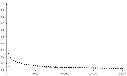
That settled, the function for randomly sampling numbers games is given in listing 15. This is a relatively straightforward implementation of our algorithm; we first randomly select a formula template, we then randomly generate a correctly sized vector of operators to substitute into it and we finally generate a random permutation of arguments. Note that we still have to copy the arguments into an appropriately sized vector since this is what our rpn_evaluate function expects. Figure 7 gives the power law graph of a sample of 40,000,000,000, or roughly 1%, of the Countdown numbers games. Once again, it looks like it tends to a straight line and the root mean square error between the line and the graph from the 24,000th to the 32,000th point of approximately 0.00035 supports this.
template<class Fun>
Fun
sample_numbers_games(size_t samples,
std::vector<long> numbers,
size_t args, Fun f)
{
typedef rpn_operator<long>
const * operator_type;
typedef std::vector<operator_type>
operators_type;
typedef std::vector<long> arguments_type;
if(args>numbers.size())
throw std::invalid_argument("");
operators_type operators(4);
const rpn_add<long> add;
operators[0] = &add;
const rpn_subtract<long> subtract;
operators[1] = &subtract;
const rpn_multiply<long> multiply;
operators[2] = &multiply;
const rpn_divide<long> divide;
operators[3] = ÷
const std::set<std::string>
templates(all_templates(args));
operators_type used_operators;
arguments_type used_arguments;
while(samples--)
{
std::set<std::string>::const_iterator t
= templates.begin();
std::advance(t,
size_t(rnd(templates.size())));
const size_t t_args = (t->size()+1)/2;
used_operators.resize(t_args-1);
random_state(used_operators.begin(),
used_operators.end(), operators);
std::random_shuffle(numbers.begin(),
numbers.end());
used_arguments.assign(numbers.begin(),
numbers.begin()+t_args);
const rpn_result<long> result
= rpn_evaluate(*t, used_operators,
used_arguments);
if(result.valid) f(result.value);
}
return f;
}
|
| Listing 15 |
|
| Figure 7 |
A theoreticalish justification
Mucking about with graphs and tests is all well and good, but it doesn't really provide any insight into the statistical behaviour of numbers games. What we really need is a theoretical justification as to why power law distributions might be reasonable approximations of them.
We shall begin by introducing yet another numbers game. In this new game we shall begin by picking, at random, a real number between 1 and 2. We shall then toss a coin; if it comes up tails the games is over and the number we picked is the result and if it comes up heads we double the number and toss the coin again, treating the doubled result as our starting point.
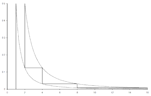
This game has a 1 in 2 chance of a result between 1 and 2, a 1 in 4 chance of a result between 2 and 4, a 1 in 8 chance of a result between 4 and 8 and so on. The probability density function of the results of this game, being the continuous limit of a histogram and for which the area under the curve between 2 values gives the probability that a result in that range will be observed, is given in figure 8. This curve is bounded by the inequality

as is illustrated by the dotted lines.
|
| Figure 8 |
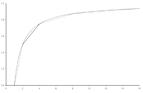
Clearly this is approximately an inverse square power law distribution. This fact is demonstrated even more clearly by the cumulative distribution function; the function that yields the area under the curve between 0 and any given value and hence the probability that we should observe a result less than or equal to that value, as illustrated in figure 9. The dotted line in this graph is the cumulative distribution function of a quantity exactly obeying an inverse square power law distribution.
|
| Figure 9 |
This result can be generalised in that a game in which we pick a real number between 1 and n and with probability p choose to multiply the current result by n rather than quit the game must also be similarly approximated by a power law distribution. Furthermore, we needn't specify which statistical distribution governs the choice of the first number for this to hold.
We can identify the first number as the relatively small result of a formula involving the addition and multiplication of relatively small numbers in the Countdown numbers game. The successive multiplications can be similarly identified with multiplying these small results by the large numbers.
Note that for each formula with n arguments, there is a formula with n +1 arguments that equates to multiplying the former by the final argument. The proportion of such formulae to all formulae with n +1 arguments is equal to
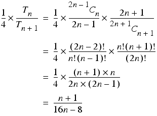
For sufficiently large n this is approximately constant, so the probability of multiplying an n argument formula by a large number is also approximately constant.
Subsequent divisions, should they be valid, can be thought of as reducing the probability of a multiplication, and subsequent additions will affect the larger results by orders of magnitude less than the multiplications.
It doesn't seem entirely unreasonable therefore to accept this latest game as an approximate model for the Countdown numbers game and that the latter can therefore be well approximated by a power law distribution.
Whilst the game is certainly not exactly governed by a power law, I believe that we can conclude with some confidence that we can reasonably approximate it with one and that there is therefore a surprising relationship between the Countdown numbers game and the recent economic meltdown.
Who'd have thunk it?
Acknowledgements
With thanks to Keith Garbutt for proof reading this article.
References and further reading
[ANSI98] The C++ Standard, American National Standards Institute, 1998.
[Clauset09] Clauset, A. et al, Power Law Distributions in Empirical Data, arXiv:0706.1062v2, www.arxiv.org , 2009.
[Countdown] http://www.channel4.com/programmes/countdown
[Harris08] Harris, R., The Model Student: A Knotty Problem, Part 1, Overload 84, 2008.
[Harris09] Harris, R., The Model Student: A Primal Skyline, Part 2, Overload 93, 2009.
[Ormerod05] Ormerod, P., Why Most Things Fail, Faber and Faber, 2005.


