Prime numbers are the 'building blocks' of the integers. Richard Harris investigates how they're combined.
The prime numbers, those positive integers wholly divisible by only themselves or by one, are perhaps the most studied numbers in all of history. Evidently a breed apart from their more mundane neighbours on the number line they are, depending upon how much number theory you have been subjected to, their noble elite, their rugged individualists, or their psychopathic loners.
Every integer can be represented as the product of a set of primes, known as the prime factors. For example the number 42 has the prime factors 2, 3, and 7 since 42 = 2 × 3 × 7.
Numbers with more than one prime factor (i.e. non-primes) are known as composite numbers and the number 1 is technically known as the identity and is neither prime nor composite.
Now, in general, the prime factors of a number may contain multiple copies of each given prime. We can capture this by raising each factor to a power representing how many times it shows up in the factorisation. For example
252 = 2 × 2 × 3 × 3 × 7 = 2 2 × 3 2 × 7 1
Noting that raising a number to the power of 0 results in 1, we can propose an alternative notation for the integers. Identifying the first, second, third and so on entries in a list as the powers to which the first, second and third and so on primes should be raised in the product, and in much the same way as we truncate trailing zeros in decimal notation, truncating trailing zeros in our list of prime powers, we have a unique representation for every integer. For example252 = 2 2 × 3 2 × 5 0 × 7 1 → 2,2,0,1
since 2, 3, 5 and 7 are the 1st, 2nd, 3rd and 4th primes.Whilst this happens to be a supremely convenient notation in which to perform multiplication, it is an atrocious notation for addition, which perhaps explains why we don't use it.
Compounding the lack of usefulness of this notation is the fact that it is actually rather difficult to identify the n 'th prime. Generally, the prime numbers are notoriously difficult to find, which is unfortunate since they lie at the heart of many of the great unanswered mathematical questions of the 21st century. Such as, for example, whether the Riemann Hypothesis is true [ duSautoy04 ], or whether it is possible to efficiently decompose numbers into their constituent prime factors [ Menezes97 ].
Euclid's proof of the infinity of the primes
It was Euclid who took the first timid steps towards subjugating these aristocrats cum robber barons of the integers by demonstrating, over two thousand years ago, that there are infinitely many of them.
His proof is elegant and simple, and as such is a rare and precious gem of number theory. It is an example of proof by contradiction in which we assume that there are only a finite number of primes and then demonstrate that this leads to a contradiction.
So, assuming there are only n primes for some undetermined value of n , we can write the product of all of them as follows:

where p i is the i 'th prime and the capital pi means the result of multiplying together all of the values from p 1 to p n . In this sense it is much like the capital sigma we use to represent the sum of a set of numbers.
Now, this number is trivially composite since it can be divided by every prime. However, consider the result of adding 1 to it:

Now, dividing this number by any of the primes leaves a remainder of 1, since the product is divisible by all of them and the 1 by none of them.
It is, by definition, greater than any of the primes in our set and hence cannot be one of them. Furthermore, since it is not wholly divisible by any of them it must either be a prime itself or have a prime factor that is not in our set. Hence our set is incomplete, no matter what value n takes and there must therefore be an infinite number of primes.
Sweet.
Having concluded that the primes are infinite in number, the next obvious question to ask is how densely packed they are amongst the integers; how many primes are there less than or equal to any given integer n ?
The prime number theorem
We have an approximate answer to this question, at least for large n , first guessed at by the mathematical giants Legendre and Gauss in the late 18th century:

The drunkenly scribed equals sign means approximately equal to, the lower case pi is the function that returns the number of primes less than or equal to its argument n and the ln is the natural logarithm; the number to which we need to raise the mathematical constant e (approximately 2.718) to recover the argument.
It took about 100 years to raise the status of this formula from conjecture to theorem, when it was tortuously proven by both Vallée-Poussin and Hadamard [ Daintith89 ].
Technically, the theorem states that the ratio between the number of primes and this formula tends to 1 as n grows larger.

The lim term here indicates that we are describing the limit of the expression that follows it as n grows larger and larger, or tends to infinity.
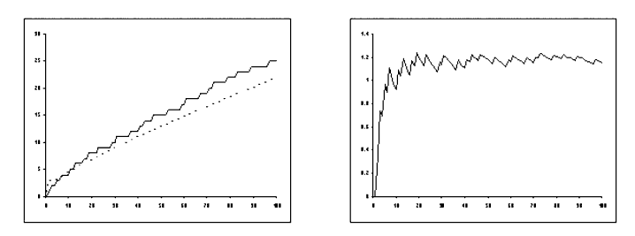
Figure 1 plots the function counting the primes as the solid line in the graph on the left, the approximation as the dotted line and the ratio between them in the graph on the right.
|
| Figure 1 |
Clearly, the approximation isn't particularly accurate in this range. Which is a shame since it could easily be used to determine the distribution of the primes amongst the positive integers, which is one of the most fundamental puzzles in number theory.
Those of you who have been following this, as it turns out rather formulaic, series of articles will not be in the least bit surprised when I abandon all attempt to address the question at hand and introduce a simpler one which I, with my limited mathematical arsenal, may actually be capable of shedding some light upon.
Ready.
Get set.
The X factors
Rather than attempt to investigate the distribution of the primes, I shall instead propose that we consider looking for a pattern in the prime factorisations of the integers. As mentioned at the start of this article, every positive integer can be represented by the product of a set of primes, with 1 being the special case of multiplying together no primes.
The simplest method of factorising integers, known as trial division, is to iterate through all of the prime numbers less than a given integer, increasing the powers of each whilst they leave no remainder upon dividing it.
Listing 1 illustrates a function that prints out the prime factors of its argument using this algorithm.
    void
    print_factors(unsigned long x)
    {
      unsigned long n = 0;
      while(nth_prime(n)<=x)
      {
        unsigned long power  = 0;
        unsigned long factor = nth_prime(n);
        while(x%factor==0)
        {
          ++power;
          factor *= nth_prime(n);
        }
        if(power!=0) std::cout << nth_prime(n) <<
           "^" << power << " ";
        ++n;
      }
    }
|
| Listing 1 |
Note that if x is sufficiently large then repeated multiplication of the factor variable by the n 'th prime might exceed the maximum representable value of an unsigned long .
Fortunately, this is not technically an overflow and hence does not invoke the dreaded undefined behaviour. This is because the C++ standard defines arithmetic with n bit unsigned integer types as being modulo 2 n , effectively throwing away any unrepresentable bits in the result of an arithmetic expression and wrapping round into the range of representable values [ ANSI ].
Unfortunately, this doesn't really help us all that much. For example, if x is equal to 2 n -1 , the result variable will eventually wrap around to 0 and the next step of the loop will involve a divide by 0 error during the modulus calculation.
Leaving this problem and the definition of the nth_prime function aside for now, we shall instead focus on some performance improvements that we can make to this approach.
The first thing we should note is that the largest repeated factor of a compound number must be no larger than the square root of that number. Indeed, if this were not so, then the product of the least possible number of repeated factors, 2, would exceed our compound number and could clearly not be equal to it.
In exploiting this fact, we must be careful that we identify any single prime factor that may be larger than the square root of the number. We can do this by keeping track of the product of the factors so far identified; if this is not equal to the original number then there must be one more unrepeated prime factor equal to the original number divided by the product of the identified factors.
Listing 2 illustrates the changes we need to make to the print_factors function to implement this improvement.
    void
    print_factors(unsigned long x)
    {
      unsigned long n = 0;
      unsigned long factors = 1;

      while(nth_prime(n)*nth_prime(n)<=x)
      {
        unsigned long power  = 0;
        unsigned long factor = nth_prime(n);

        while(x%factor==0)
        {
          ++power;
          factor  *= nth_prime(n);
          factors *= nth_prime(n);
        }

        if(power!=0)  std::cout << nth_prime(n)
           << "^" << power << " ";
        ++n;
      }

      if(x!=0 && factors!=x) std::cout << x/factors
         << "^1 ";
    }
|
| Listing 2 |
Unfortunately, we have introduced another sensitivity to integer wrap around. If x is sufficiently large then the square of the smallest prime strictly greater than it could wrap around. This means that we may very well enter into an infinite loop, never finding a prime whose square, modulo 2 to the power of the number of bits in an unsigned long , is greater than x .
Ignoring this potential problem too, we finally note that even if we have found all of the factors of the number we will still keep looking until we reach the last prime less than or equal to its square root.
A further improvement is therefore to divide the number by each factor we discover, allowing us to stop when we reach a prime larger than the square root of the product of the remaining factors, if any.
If this remaining product is anything other than 1, it must be a single non-repeated prime factor. To prove this, recall that every compound number must have at least one factor no greater than its square root and since we have already removed all such factors it cannot therefore be a compound number.
This final change to the trial division algorithm is illustrated in listing 3.
    void
    print_factors(unsigned long x)
    {
      unsigned long n = 0;

      while(nth_prime(n)*nth_prime(n)<=x)
      {
        unsigned long power = 0;

        while(x%nth_prime(n)==0)
        {
          ++power;
          x /= nth_prime(n);
        }

        if(power!=0)  std::cout << nth_prime(n)
           << "^" << power << " ";
        ++n;
      }

      if(x>1)  std::cout << x << "^1 ";
    }
|
| Listing 3 |
The performance improvement from this change is significantly less dramatic than that of the first, as illustrated in figure 2, which gives the time each version of the algorithm takes to factor (but not print) the integers from 2 to 100 using the machine with which I happen to be writing this article 10,000 times each.
|
|
||||||
| Figure 2 |
That said, it does neatly side step the possible wrap around issue whilst multiplying the factor variable by the n 'th prime, although it does not address that of squaring the n 'th prime.
The n'th prime
So, given that we don't have an exact formula for the n 'th prime, how are we to go about implementing the nth_prime function?
To be perfectly honest, we can't; the function I used to test the various implementations of the print_factors function used a look up table of the primes between 0 and 100, which I'm sure you'll agree isn't particularly scalable.
However, if we are interested in the factorisations of all numbers up to a given upper bound, which I can assure you we shall be, we can build the table of primes as we go.
Instead of providing a function to calculate the primes, we will provide a pair of iterators that range from the first prime, 2, to a prime guaranteed to be no smaller than the square root of the number we seek to factor. Furthermore we change the function to return a bool to indicate whether or not the number in question remained unchanged throughout the trial division and is itself therefore a prime
Listing 4 illustrates the changes we need to make to the print_factors function.
    template<class FwdIt>
    bool
    print_factors(unsigned long x, FwdIt first_prime,
       FwdIt last_prime)
    {
      const unsigned long x0 = x;

      while(first_prime!=last_prime &&
         (*first_prime)*(*first_prime)<=x)
      {
        unsigned long power = 0;

        while(x%*first_prime==0)
        {
          ++power;
          x /= *first_prime;
        }

        if(power!=0)  std::cout << *first_prime
           << "^" << power << " ";
        ++first_prime;
      }

      if(x>1)  std::cout << x << "^1 ";
      return x0>1 && x==x0;
    }
|
| Listing 4 |
We can now supplement this with a second function that iterates from 0 (or strictly speaking a non-negative number less than or equal to 2) up to some upper bound printing the factorisation of each of them.
This second function can use the result of print_factors to add new primes, up to the square root of the upper bound, to the back of the sequence that the iterators range over.
Note that we can use the prime number theorem to get an estimate of how large the sequence of primes might be. By multiplying this estimate by some constant factor sufficiently greater than 1, we can ensure that it will exceed the number of primes in almost all cases. This, in turn, ensures that in almost all cases we can reserve enough space for all of the primes we'll need in a std::vector . Of course, this is a ridiculous micro-optimisation, but we shall eventually be desperate for simple ways to squeeze out those last few wasted cycles.
Moving on from that rather vague justification for my apparent performance anxiety, we shall implement this as an overload of the print_factors function as illustrated in listing 5.
    void
    print_factors(unsigned long upper_bound)
    {
      std::vector<unsigned long> primes;

      const double pi_upper_bound =
         sqrt(double(upper_bound)) /
         log(sqrt(double(upper_bound)));

      const unsigned long n(1.5*pi_upper_bound);
      primes.reserve(n);

      unsigned long x = 1;
      while(x<upper_bound)
      {
        std::cout << x << ": ";
        bool is_prime =
           print_factors(x,primes.begin(),
           primes.end());
        std::cout << std::endl;

        if(is_prime && x*x<=upper_bound)
           primes.push_back(x);
        ++x;
      }
    }
|
| Listing 5 |
Note that this function too suffers from potential integer wrap around whilst squaring prime numbers when we're checking whether to add them to our list.
The output of this function for the integers from 1 to 20 is given in figure 3. Note that since 1 is neither prime nor compound, it has no factors.
    1:
    2: 2^1
    3: 3^1
    4: 2^2
    5: 5^1
    6: 2^1 3^1
    7: 7^1
    8: 2^3
    9: 3^2
    10: 2^1 5^1
    11: 11^1
    12: 2^2 3^1
    13: 13^1
    14: 2^1 7^1
    15: 3^1 5^1
    16: 2^4
    17: 17^1
    18: 2^1 3^2
    19: 19^1
    20: 2^2 5^1
|
| Figure 3 |
Omega? Feh!
Now, analysing the complete factorisations of ranges of integers is something of a tall order, so instead I suggest we simply count how many prime factors each integer has. A cousin of the prime counting function P , the function that returns the number of prime factors (including repeated factors) of its argument is denoted by Ω .
Using the factorisations we calculated in figure 3, and noting that 0 is the result of dividing 1 by infinitely many factors, we can derive the values of Ω for the integers from 0 to 20, as illustrated in figure 4.
|
|
|||||||||||||||||||||||||||||||||||||||||||||||||||
| Figure 4 |
This function has some useful properties, not least of which is that it maps non-negative integers to integers, assuming we're happy to count negative infinity as an integer. Furthermore, every number for which this function evaluates to 1 is, by definition, a prime; it has, after all only 1 prime factor.
It would be extremely tedious to work out the values of Ω from the factorisations we can currently produce. Fortunately, we can simply adapt the functions to count the factors instead. Listing 6 illustrates the function to count the factors of a single integer.
    template<class FwdIt>
    unsigned long
    count_factors(unsigned long x, FwdIt first_prime,
       FwdIt last_prime)
    {
      unsigned long count = 0;

      while(first_prime!=last_prime &&
         (*first_prime)*(*first_prime)<=x)
      {
        while(x%*first_prime==0)
        {
          ++count;
          x /= *first_prime;
        }

        ++first_prime;
      }

      if(x>1)  ++count;
      return count;
    }
|
| Listing 6 |
We shall overload this to count the factors of every positive integer up to some upper bound, in much the same way as we did for print_factors . The single integer function no longer returns a bool to indicate that the argument is a prime, but as noted above if a number has precisely 1 factor it must be prime and we can use this fact as the indication that we should add the number to the back of our sequence of primes. This second function is given in listing 7.
    void
    count_factors(unsigned long upper_bound)
    {
      std::vector<unsigned long> primes;

      const double pi_upper_bound =
         sqrt(double(upper_bound)) /
         log(sqrt(double(upper_bound)));
      const unsigned long n(1.5*pi_upper_bound);
      primes.reserve(n);
      unsigned long x = 1;
      while(x<upper_bound)
      {
        const unsigned long count = count_factors(
           x, primes.begin(),primes.end());
        std::cout << x << ": " << count << std::endl;
        if(count==1 && x*x<=upper_bound)
           primes.push_back(x);
        ++x;
      }
    }
|
| Listing 7 |
The output of this function for the integers from 1 to 20 is given in figure 5, which you can see is in agreement with our hand derived values for Ω .
1: 0 2: 1 3: 1 4: 2 5: 1 6: 2 7: 1 8: 3 9: 2 10: 2 11: 1 12: 3 13: 1 14: 2 15: 2 16: 4 17: 1 18: 3 19: 1 20: 3 |
| Figure 5 |
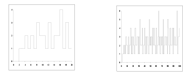
The graphs of Ω for the integers from 1 to 20 and from 1 to 100 are given in figure 6. We extend this from the integers to the real numbers by plotting the value of Ω for the integer part of each real number.
|
| Figure 6 |
It is tempting to look for patterns in these graphs and there is, in fact, a particularly striking one. To see it we need to look at an exponential function of Ω ; specifically raising 2 to its power.
In keeping with the time honoured tradition of naming mathematical functions with single letters from non-Latin alphabets, I christen this function ף n .


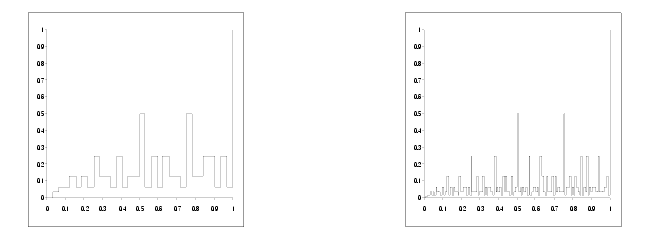
You may recall from previous articles that the odd square brackets surrounding the 2 n x terms means the largest integer less than or equal to the value between them and that the expression on the right with the rounded E means that x must be in the range 0 to 1. Figure 7 illustrates the graphs of ף 5 and ף 7 .
|
| Figure 7 |
The properties of ף n
For any n , ף n is defined for arguments between 0 and 1. Moreover, at 0 it returns a value of 0 and at 1 it returns a value of 1.
To demonstrate this, we note firstly that for x equal to 0, Ω receives an argument of 0 and returns negative infinity. Since any number greater than 1 raised to negative infinity yields 0, ף n returns 0 for an argument of 0.
Secondly, the integer between 0 and 2 n with the most factors is 2 n , since 2 is the smallest prime. This has n factors and hence the top and bottom of the fraction defining ף n are equal when x equals 1, yielding a result of 1.
In fact, the entire graph must never rise above the line from (0,0) to (1,1) as proven in derivation 1.
|
First we assume that the graph can rise above the line and show that this leads to a contradiction. This assumption means that for some x 
implying that 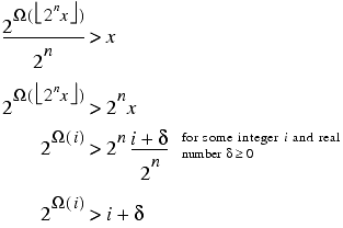
Now, since the left hand side of the inequality is an integer and is greater than or equal to 0, we have 
Of course, this is impossible since 2 is the smallest prime number and hence must be less than or equal to 2 Ω( i ) and consequently ף n ( x ) must be less than or equal to x . |
| Derivation 1 |
Another statement that we can make about these curves is that for all n greater than 0, ף n must coincide with ף n -1 for half of the values of x ; specifically, those where the integer part of 2 n x is even, as demonstrated in derivation 2.
|
Noting that ⌊ a ⌋ = 2 × ⌊½ a ⌋ for even ⌊ a ⌋, for even ⌊2 n x ⌋ we have 
|
| Derivation 2 |
The curves ף n and ף n -1 are further related by the equation

as shown in derivation 3.
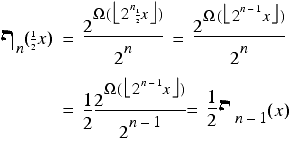
Note that since we haven't exploited the properties of Ω , this would hold if we replaced it with any other function. |
| Derivation 3 |
If we combine these two properties then we recover the striking pattern that I alluded to above; specifically that, when the integer part of 2 n x is even, we have

Now this may not strike you as being especially striking, but it is strikingly similar to a property exhibited by many of a very well known class of curves; the fractals.
Many fractals are defined in terms of a sequence of curves which serve as closer and closer approximations to the fractal itself. These curves can themselves be approximated by zooming in on sub-sections of them, in much the same way as we can for ף n . The major difference is that for the iterative approximations of fractals we can zoom in on many parts of the curve rather than just one specific region.
We can uncover further hints at the relationship between fractals and ף n by considering the limit as n tends to infinity. Waving our hands somewhat vigorously we can take the result that

and infer that

since ף n -1 is approximately equal to ף n for arbitrarily accurate interpretations of approximately.
Now, instead of recovering an approximation of the curve by zooming in on a sub-section of it, we can entirely reconstruct it. Specifically, for all values of x , we have

This is suspiciously similar to the self-similarity property of many fractals; the ability to reconstruct the entire curve by zooming in on sub-sections of it.
So is ף ∞ itself a fractal?
Well, that happens to be a very interesting question and we shall pursue its answer in the next article.
Until then, dear reader, fare well.
Acknowledgements
With thanks John Paul Barjaktarevic and Lee Jackson for proof reading this article.
References and further reading
[ANSI] The C++ Standard, American National Standards Institute
[Daintith89] Daintith, J. & Nelson, R. (ed), The Penguin Dictionary of Mathematics, Penguin, 1989
[duSautoy04] du Sautoy, M., The Music of the Primes, Harper Perennial, 2004.
[Menezes97] Menezes, A. et al, Handbook of Applied Cryptography, CRC Press, 1997


