Divide and Conquer: Partition Trees and Their Uses

Partition trees are a useful data structure for maintaining a hierarchy of partitions of an entity, e.g. the world, an image, or even a pizza. In this article, I want to explain how they work and describe some of their uses.

A partition of an entity is a division of it into mutually disjoint parts which together make up the whole entity. (Put mathematically, a partition of E is a set S = {E1,...,En} of sub-entities of E such that Union(S) = E and for all i,j in {1,n}, i != j → intersect(Ei, Ej) = ∅.) For example, we could partition a pizza into twelve slices: none of the slices overlap, and together they make up the whole pizza (until someone starts munching, at any rate).

A partition tree is a way of representing a hierarchy of these partitions of an entity. The way it works is as follows:

• Each node in the tree represents a part of the whole entity. In particular, the root node of the tree represents the entity in its entirety.
• As is usual with trees in computer science, a node is either a branch node or a leaf node. (The distinction is that a branch node has child nodes, whereas a leaf has none.) In a partition tree, the children of a branch node represent a partition of the branch node (properly speaking, the parts of the entity represented by the children of the branch node represent a partition of the part of the entity represented by the branch node, but continually distinguishing between nodes and the sub-entities they represent is tedious).
• Each layer in the hierarchy represents a partition of the entire entity.

Using our pizza analogy, we could imagine first dividing our pizza into three portions, one for each person at the table. Each person's portion is then further sub-divided into four slices. Each person's slices are a partition of their portion, and the portions are a partition of the pizza as a whole. Furthermore, if you take all the slices, or all the portions, together, you have the entire pizza.

As a graphical example, take a look at Figure 1, which shows a partition tree for the square image shown at the bottom-right. The image pieces at each node are colour-coded for easy identification in the images for each layer of the tree on the right. They are clearly mutually disjoint, and their union in each case is the whole image. This example with images illustrates one potential use for partition trees (and indeed the reason I'm interested in them at the moment, as those of you who saw my previous articles on image segmentation [ Golodetz08b ] may have guessed), but it is very much one among many.

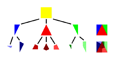
Figure 1

Binary space partitioning

We'll return to image partition trees later, but first I want to look at a different domain in which partition trees are useful, that of partitioning 2D or 3D space. Space partitioning is an extremely useful tool in the arsenal of 3D graphics programmers, particularly in the context of games, which was where I first encountered the technique.

The general idea is to start with an infinite space (e.g. the game world) and recursively divide it into pieces. This division can happen in a number of ways, depending on the type of tree, but we'll start by discussing binary space partitioning .

Binary space partitioning, as its name suggests, is the process of recursively dividing a world into two. We start with our infinite world, split it across a plane, then split the newly formed sub-spaces on each side across other planes, and carry on until we run out of sub-spaces we want to split. These terminal sub-spaces become the leaves of our tree. (Figure 2 shows an example of the BSP construction process.) Each branch node stores the plane which was chosen to split its sub-space into two (the splitter , or split plane ), and the tree generally satisfies the property that every node in the sub-tree rooted at the left child of a branch node represents a sub-space in front of that branch's splitter, and conversely for nodes in the right sub-tree. One consequence of the way the splitting process works is that the sub-spaces represented by the nodes are all convex (inductive proof: the initial world can be viewed as convex, and splitting a convex space across a plane gives you two convex sub-spaces as a result).

The BSP construction process for a simple L-shaped room: at each stage, a split plane is chosen to split the world in two, according to a metric m based on the weighted linear combination of the balance of polygons on either side of the splitter and the number of polygons which will be split if that splitter is chosen. The plane of a polygon with the lowest value of m is chosen. The value of m in the figure is calculated as 8*| front - back | + 1* straddle , where front is the number of polygons completely in front of the plane, back is the number completely behind, and straddle is the number straddling the plane. The weights 8 and 1 are somewhat arbitrary, and the ratio between them can be varied to produce alternative trees.

Figure 2

As an example of this, consider Figure 3. In (a) we see the recursive partitioning of a 2D world consisting of two rectangular rooms joined by a short corridor, whilst (b) shows its equivalent partition tree. Branch nodes in the tree are marked with the number of the wall they correspond to in (a), while leaf nodes are marked either ^ or T (along with a Greek letter indicating the convex subspace in (a) to which they correspond). Leaves marked ^ are called empty leaves, and represent the parts of the world which are inside the rooms/corridor (the bits a player could walk around in, were this a game). Leaves marked T are called solid leaves, and represent the opposite.

A partition diagram of an example 2D world (above) and its partition tree (below).

Figure 3

So why is this representation useful? Well, for a start, a tree like this can easily answer the question of whether any given point is in empty or solid space. As those of you who can remember your maths will recall, the equation of a plane is:

where n is the unit normal of the plane, x is an arbitrary point on the plane and d is the plane distance value. The plane normal indicates the facing of the plane. Plugging a specific point x into this equation gives us a positive value if x is in front of the plane, a negative value if it's behind, and 0 if it lies in the plane (when we call it a coplanar point).

We can therefore classify a point in terms of where it lies in relation to a plane. To determine whether a point lies in empty or solid space, we start by classifying it against the split plane for the root node of the tree. If it lies in front of the plane, we recurse to the left child of the root (the child representing the sub-space in front of the plane) and classify the point again; if behind, we recurse to the right child. (If it lies on the plane, we have a choice of what to do: if we recurse down the front side of the tree, then coplanar points will be classified as being in empty space; if we recurse down the back side, they'll be in solid space. It's up to us in this case.)

Eventually we will recurse into a leaf, which has no split plane. At this point, we return whether or not the leaf is solid as the result. This method provides a simple (if very naive) way of doing collision detection for small objects: we move an object, check whether its centroid is in solid space, and perform collision resolution on it if so. (There are much better ways, however!)

Another simple technique can be used to find the first 'transition point' of a half-ray, i.e. the first point at which the half-ray first goes from empty space to solid space, or vice-versa (the first point at which it hits a wall). (Specifically, given a ray r (λ) = start + λ( dir ), λ ≥ 0, the algorithm will return the transition point closest to start .) The process essentially works in a similar way to a line segment classifier, but it prioritises the side of the tree nearest the start of the ray. Starting from the root of the tree, the algorithm classifies the ray against the split plane at the current node (via classifying its endpoints against the plane). If it is entirely on one side of the plane, it is passed down the relevant side of the tree. If it straddles the plane, it is split in two at the plane and the two halves are passed down their respective sides of the tree, with the half nearest the start of the ray being processed first and the other half only being processed if no transition point has been found in the first half. Finally, there are a number of annoying coplanar special cases: I don't want to get into those here, but the interested reader can find working code for the whole algorithm in my transfer report [ Golodetz08a ]. The find first transition algorithm provides a way of testing 'line-of-sight' in a game world (although it actually gives you back more information than you strictly need, as line-of-sight is a boolean value): this can be useful for AI players when deciding whether to try and shoot you, for example. It can also provide a (slightly!) better method of collision detection than the point-checking method above: we check whether the ray from the object's old location to its new location intersects a wall, and move it back to somewhere near the first transition point if it does (I say 'somewhere near' because we're usually dealing with objects that have extent, rather than point objects).

As a brief aside, I'll quickly mention a reasonably good BSP-based collision detection scheme you can use for objects with extent. This was used in id Software's Quake III Arena [ VanWaveren01 ], with good results. The basic idea is a configuration space one. They determine an axis-aligned bounding box for each class of object in the game, then generate a special collision BSP for each size of bounding box (not necessarily one for each class of object, though this can happen if all the classes have different bounding boxes). Quake III worlds are built up from a large number of convex building blocks (brushes). In order to build a collision BSP for a particular size of bounding box, they push the planes which define each brush along their respective normals by a certain amount (thus expanding the brush anisotropically ). Each plane is moved along its normal by the amount which would take it to the centre of the bounding box when the box was just touching the plane (see Figure 6.4 in [ VanWaveren01 ] for a picture). The collision BSP is then built from the expanded brushes. What this whole exercise achieves is the generation of a tree that defines where the centroid of bounding box is allowed to go (i.e. the configuration space for the centroid): an annoying bounding box collision detection problem has thus been reduced to a point problem. We can then use any scheme we like (e.g. the find first transition approach described above) to perform the actual point-based collision detection. It should be noted that there are a few complications to the whole approach, which are described in [ VanWaveren01 ], but this is the basic principle involved.

Collision detection aside, BSP trees are also useful for rendering. They provide us with a way to render our polygons in back-to-front order when viewed from an arbitrary position in the world. This was especially useful in the days when z-buffers were still quite costly to use, but it remains a useful technique even now when rendering transparent polygons. The rendering algorithm is once again recursive:

• Starting from the root node, classify the position of the viewer against the split plane.
• If it's in front of the plane, recurse down the back half of the tree and render all the polygons behind the plane, then render the polygon on the plane itself, then recurse down the front half of the tree and render all the polygons in front of the plane.
• If it's behind the plane, do the opposite, except that the polygon on the plane itself isn't rendered (we're behind it, so it gets back-face culled).

One very useful thing you can do with BSP trees (which saw use in id Software's Quake [ Abrash97 ]) is to precalculate something called the potentially visible set (PVS) of each leaf in the tree. This basically means calculating and caching which leaves can be viewed from which other leaves. The way this is done is a little bit complicated, but the first step is to calculate all the portals (doorways) between the various leaves: an interesting and useful process in itself. Portal calculation essentially involves clipping polygons to the tree. We build massive polygons (bigger than our game world) on each unique plane in which one of our world polygons lies, then clip them to the tree to get the portals. Caching the PVS for each leaf makes rendering substantially (e.g. an order of magnitude) faster. Instead of having to render all the polygons in the game world, we now only have to render a small subset of them. This was one of the key techniques that made Quake run so fast.

A final BSP-related technique worth mentioning is that of constructive solid geometry (CSG). This is a completely general technique which involves combining primitive solid objects into more complicated ones using set operations (i.e. union, intersection and difference) and doesn't necessarily have to be implemented using BSP trees, but doing CSG using BSP trees works rather well. Figure 4 shows the idea: by combining two simple squares together, we can create a hollow square using a difference operation. This sort of approach works extremely well in game level editors, since it allows the user to create complicated worlds from a very simple set of initial objects (e.g. cuboids, cylinders, cones and spheres). For more details, see my undergraduate project report [ Golodetz06 ].

A simple example of a CSG difference operation

Figure 4

Quadtrees and octrees

For now, let's look at a completely different way of partitioning the world. Quadtrees (in 2D) and octrees (their 3D analogue) are a way of sub-dividing the world along axis-aligned planes. Consider Figure 5, in which we imagine applying a quadtree approach to a 2D map of a river running through a landscape. The idea is basically as follows: at each stage, we divide the space into four along planes in the x and y directions. We have some sort of termination criteria to tell us when to stop. For instance, we could stop dividing a square when it contains > 95% river or land, say.

An example quadtree for a river - only the first 5 levels are shown.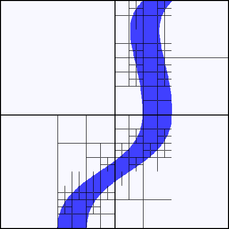

Figure 5

So why is this useful? One obvious application is mesh generation: if we've got large homogeneous areas of land, such as in the north-west part of the image, we don't want to generate a fine mesh for them because it's wasteful. If there's a lot of detail, however, such as in the north-east of the image, we don't want to miss it by having too coarse a mesh. Quadtrees provide one solution to this problem (another would be a binary triangle tree algorithm like ROAM - real-time optimally adapting meshes [ Duchaineau97 ]) by effectively adapting the grid size to the local terrain.

As with BSP trees, quadtrees can be used to classify a point in the world: in this case, we can easily determine whether a given point is part of the river or part of the terrain by recursively classifying the point against the tree. 'Big deal!', you might think, since we have the original image and can just look it up in that. But quadtrees are a much more space-efficient representation of the world than the original image: this allows us to capture the useful information in the original image without keeping it continually hanging around in memory.

There are lots of other uses of quadtrees besides dividing the terrain. One such application is collision detection (see Figure 6). The idea of Figure 6 is basically that objects can only collide with objects in the quadrants they are in. So for instance, the square object won't collide with the stationary circles elsewhere in the world, so we don't need to check for that. There's more to it than that, of course, such as how to change the tree when the objects move around, but that's another story.

Using a quadtree to avoid doing unnecessary collision detection - the square remains within its quadrant, so it will never collide with the stationary circles and doesn't need to be tested against them.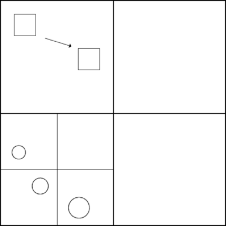

Figure 6

Image partition trees

For now, I want to conclude this brief overview of partition trees by returning to the image partition trees (IPTs) we started with in the introduction. So far, the partition trees we've seen have been constructed using a top-down splitting approach. This is certainly possible for IPTs, but for the purposes of this article, I want to describe an alternative bottom-up approach based on region merging.

The basic plan is as follows. We start by somehow generating a large number of small regions in the image, then combine some of them to form the next layer up in the tree, then iteratively repeat this process until we run out of regions to merge (i.e. we get a single region at the top of the tree: the root). At a more concrete level, the algorithms I described in my previous articles [ Golodetz08b ] can be directly put to use here: the watershed transform will give you a very fine initial partition of the image into small regions, and the waterfall algorithm can be used for the actual merging process, thereby generating a hierarchy of partitions of the image that get coarser the further up the tree you get. (Other approaches can also be taken here: this is merely by way of an 'existence proof' that it can be done.)

Having generated an IPT, what can we do with it? Its main use (i.e. its advantage over the simple sequence of partitions generated as the normal output of the waterfall algorithm) is in representing how regions were merged: it's very useful to know that (say) a kidney and two bits of liver were merged into a larger region, since if we identify the kidney (a process which will remove it from consideration) then we know that the remainder of the larger region represents the liver. It's also useful for knowing about parent relationships: if two regions are good candidates for being identified as a kidney, it's very important to know if one is the parent of the other, since it helps us distinguish between there being two separate kidneys, and there being two different versions of the same kidney.

Conclusion

Partition trees are a hugely useful information representation in at least two different domains. In this article, I've done my best to give you a broad overview of the various uses of spatial partition trees for things like collision detection, rendering, constructive solid geometry, mesh generation, and the use of image partition trees for feature identification in images. In future articles, I hope to return to a few of the topics, such as portal and PVS generation, and level building using CSG, in more detail.

Till then...

References

[ Abrash97] Abrash, M., Graphics Programming Black Book (Special Edition), Coriolis Group Books, July 1997.

[ Duchaineau97] Duchaineau, M., et al., 'ROAMing Terrain: Real-time Optimally Adapting Meshes', IEEE Visualization Journal , 1997.

[ Golodetz06] Golodetz, S., A 3D Map Editor (undergraduate project report), May 2006: http://compsci.gxstudios.net/project.pdf.

[ Golodetz08a] Golodetz, S., Segmentation of Abdominal Organs and Growth Modelling of Tumours in Renal Cancer Patients , (transfer report), p.59, May 2008: http://dphil.gxstudios.net/transfer2.pdf.

[ Golodetz08b] Golodetz, S. 'Watersheds and Waterfalls', Overload 83/84 , February/April 2008.

[ VanWaveren01] Van Waveren, J.M.P., The Quake III Arena Bot , (MSc Thesis), p.25 onwards, June 2001: http://www.kbs.twi.tudelft.nl/docs/MSc/2001/Waveren_Jean-Paul_van/thesis.pdf.