Tying yourself in knots is easy. Richard Harris cuts through the complexity.
Last time we took a look at the number of self crossings of a random walk with the intention of shedding some light on why headphone cables and the like behave so malevolently. We developed some code to exhaustively search through all possible walks of a given length, but as is often the case this gets computationally burdensome for large problems. What we really need is to find a formula for the expected number of self crossings which we will hopefully be able to exploit to deduce the likelihood that a walk will contain any given number of crossings, or to use the technical term, the distribution of crossings.
To that end, the first thing we should observe is that it is relatively easy to calculate the probability that a walk of n steps will end at its starting point. It is simply the probability that the number of steps to the left is equal to the number of steps to the right and the number of steps forward is equal to the number of steps back [ Feller, 68 ].
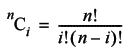
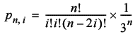
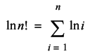
To construct the formula we need to derive an expression for the probability that a walk of n steps will have exactly i steps to the left and right, or equivalently forward and backward.
If we didn't allow a step to leave the walk in the same place, the number of ways we could have i steps to the left, and hence n - i steps to the right, would simply be the number of ways we could choose i from n things, given by the combination formula:
The probability that these numbers of left and right steps occur is determined by the binomial distribution. To calculate it we need only multiply the number of ways it can occur by the probability of each of those ways.
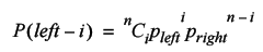
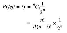
Since we have an equal probability for each kind of step, this simplifies to
The probability that we will take i steps to the left, j steps to the right and hence n -( i + j ) non moving steps is given by the related trinomial distribution.
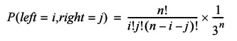
So the probability that we return to the start with exactly i steps to the left and right is given by
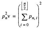
Therefore the probability that we return to the starting point after n steps, at least in one dimension, is simply the sum of the probabilities that with return with every possible number of steps to the left and right. These range from zero up to ½ n .
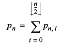
The weird brackets at the top of the summation mean the largest integer less than or equal to ½ n , by the way.
To transform this into the probability that we return to the starting point in two dimensions we need only observe that the probabilities in each dimension are independent; the likelihood of our being in the same place horizontally has no bearing on the likelihood of our being in the same place vertically. We can therefore simply multiply the two, identical as it happens, probabilities.
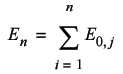
The next step in our derivation is to deduce the expected number of times a walk will return to its starting point. This is simply one times the probability that it returns after one step plus one times the probability that it returns after two steps and so on. In other words we simply sum the probabilities from the first to the last step.
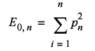
The final step is to note that at each point in the walk, we can consider ourselves to be at the starting point of a shorter walk. The total expected number of knots should therefore be the sum of the expected number of returns for every walk from one to n -1 steps.
Unfortunately we're going to run into a few problems calculating this number. The factorial at the heart of the formula is an O( n ) operation and thus the entire calculation is O( n 4 ); a rather daunting task. Furthermore, as was pointed out in the analysis of the travelling salesman problem, the factorial grows very quickly as its argument increases. Very, very quickly; 13! is too large to fit into a 32 bit unsigned integer and at 171! we'll exceed the maximum value of an IEEE 64 bit floating point number.
We can address the latter problem using logarithms. As you are no doubt aware, the logarithm of a product is equal to the sum of the logarithms of its terms.
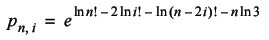
Since the trinomial distribution divides an n ! term by three factorial terms and a further 3 n term, we can be confident that it will not overflow as quickly as the terms n ! will. We will be therefore better off working with log factorials and inverting the logarithm at the end. The inverse of the logarithm is the exponential function; we can recover the final value by taking the exponential of its logarithm. Exploiting the remaining properties of logarithms, we have
The former problem can be mitigated with judicious use of caching. Both the log factorial and the probability of return, p n 2 , are calculated multiple times for the same arguments. If we cache the results of p n 2 we can reduce the complexity of the calculation by two orders of magnitude to O( n 2 ); much less daunting. Caching the results of the log factorial similarly reduces the cost of calculating p n 2 . This only results in a further constant factor improvement in efficiency, but will probably be useful in future, so we might as well implement it.
When we need a log factorial not already in the cache, we can exploit the fact that we have already done some of the work. Rather than iterate all the way from one to n , we need only work our way up from the greatest value we already have, populating the intervening entries in the cache on the way (Listing 1).
    namespace knots
    {
      double log_factorial(size_t n);
    }

    double
    knots::log_factorial(size_t n)
    {
      static std::vector<double> results(1, 0.0);
      if(n>=results.size())
      {
        size_t i = results.size();
        results.reserve(n+1);
        while(i!=n+1)
        {
          results.push_back(
             results.back() + log(double(i++)));
        }
      }
      return results[n];
    }
|
Listing 1 |
As it stands the cache could grow uncontrollably, severely reducing the efficiency of the function. If we were planning to use this as a general purpose algorithm we should probably address this problem. One approach would be to set a fixed upper limit, after which we return infinity (Listing 2).
    double
    knots::log_factorial(size_t n)
    {
      static const size_t max_n = 2047;
      if(n>max_n)
        return std::numeric_limits<double>::infinity();
        ...
    }
|
Listing 2 |
The problem with this is that it puts an artificial limit on the maximum factorial we can calculate. Fortunately, there is an approximation we can use instead; a (relatively) modern improvement [ Robbins, 55 ] on a long standing approximation known as Stirling's formula.
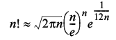
For values of n greater than a few thousand or so, the relative error in the logarithm of this approximation is of the order of 10 -12 , which is probably sufficient for our needs (Listing 3).
    double
    knots::log_factorial(size_t n)
    {
      static const size_t max_n = 2047;
      static const double pi = 2.0*acos(0.0);
      if(n>max_n)
      {
        return 0.5*log(2.0*pi*double(n)) +
               double(n)*(log(double(n))-1.0) +
               1.0 / (12.0 * double(n));
      }
      ...
    }
|
Listing 3 |
An exact value can be derived for all n , up to numerical overflow at least, from the Gamma function. This is a fundamental mathematical function that crops up in a variety of situations and is defined by
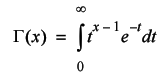
Unfortunately it has no closed form solution. It can be approximated numerically, Press et al [ Press, 92 ] provide an implementation, but it's not particularly straightforward so I'm going to stick with Stirling's formula.
The next step is to implement a function to calculate the probability of return, p n 2 (Listing 4).
    namespace knots
    {
      double p_returns_after(size_t n);
    }

    double
    knots::p_returns_after(size_t n)
    {
      static std::vector<double> results(1, 0.0);
      if(n>=results.size())
      {
        size_t i = results.size();
        results.reserve(n+1);
        while(i!=n+1)
        {
          double next = 0.0;
          for(size_t j=0;2*j<=i;++j)
          {
            double term = log_factorial(i)
                        - 2*log_factorial(j)
                        - log_factorial(i-2*j)
                        - double(i)*log(3.0);
            next += exp(term);
          }
          next *= next;
          results.push_back(next);
          ++i;
        }
      }
      return results[n];
    }
|
Listing 4 |
Once again, we simply resize the cache if we get a request for a value we have not yet calculated and populate it for all values up to the one we need. Unfortunately, this time there's no approximation we can rely on to restrict the growth of the cache. Since this function isn't really useful outside of this analysis we don't have to take possible future applications into account, so it doesn't present quite so much of a problem as it did for the log factorial calculation.
Most of the work is done in the inner loop; it is simply the calculation of p n . As discussed we use log factorials to calculate the log of each term and take the exponential at the end in order to avoid overflow. Finally, we square the probability to transform it to two dimensions before storing it in the cache.
We finally have the scaffolding in place to calculate the expected number of knots. The last two functions we need to implement are E0, n and En and, fortunately, both are relatively simple. They are illustrated in Listing 5 (which is calculating the expected proportional number of knots) and, in keeping with what they represent,we refer to E 0, n as expected_returns_to_start and E n as expected_knots .
    namespace knots
    {
      double expected_returns_to_start(size_t n);
      double expected_knots(size_t n);
    }

    double
    knots::expected_returns_to_start(size_t n)
    {
      double result = 0.0;
      for(size_t j=1;j!=n+1;++j)
         result += p_returns_after(j);
      return result;
    }

    double
    knots::expected_knots(size_t n)
    {
      double result = 0.0;
      for(size_t i=1;i!=n+1;++i)
      {
        result += expected_returns_to_start(i);
      }
      return result / double(n);
    }
|
Listing 5 |
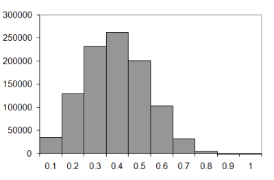
So how does this function compare to the observations we've already made? Not very well as it happens (Figure 1):
|
|||||||||||||||
| Figure 1 |
Congratulations to those of you who've already spotted the error in my reasoning; it took me a while to figure it out. The problem is that when we add up the expected number of returns, we're not taking into account the probability that we've already visited the current position.
To illustrate this point imagine that a random walk has returned to the starting point on the second step. We should not therefore include the expected number of returns to the second point in the calculation; since it is the starting point they have already been accounted for. Unfortunately this over-count occurs whenever we return to a point we have already visited during a given walk. Quite frankly, it's surprising that the approximation isn't much, much worse.
A further irritation is that I can't quite see how to figure it into the calculation. We can make some progress by observing that a random walk looks the same both forwards and backwards. The probability that the n th step is into a previously unvisited position is therefore equal to the probability that we never return to the starting point in an n step random walk. This can be expressed with a conditional probability; it is the probability that the n th step doesn't return to the start given that none of the previous steps have. This naturally recursive property could be used to construct the desired result. Well, it could if I could work out what the value of the conditional probability actually is.
Formally, the conditional probability of an event A occurring given that an event B already has is given by
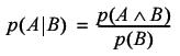
I should point out that the caret like symbol is one of the mathematical representations of 'and'.
If the events A and B are independent then the probability of them both occurring is simply the product of the probabilities of each of them occurring. The conditional probability then simplifies to:
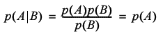
The trouble is, our steps are not independent, and their mutual dependence is too complicated for me to express the conditional probability mathematically.
We can, however, try to approximate the expected number of returns by assuming that the steps are independent, allowing us to simply multiply the probabilities that each remaining step does not return to the current position.
We already have an expression for the probability that a step does return. The probability that it doesn't is simply this value subtracted from one. The probability that the n th position is unique is therefore
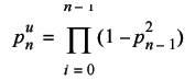
I'm using the u superscript to distinguish this probability of uniqueness from that of a walk returning to its starting point.
The giant Π is the mathematical notation for the product of a series of terms and is analogous to the use of Σ to represent sums. In fact they were both chosen because they are the Greek versions of the first letters of product and sum, respectively.
The implementation is pretty straightforward as Listing 6 illustrates, which calculates the probability that a step enters an unvisited position.
    namespace knots
    {
      double p_is_unique(size_t n)
    }

    double
    knots::p_is_unique(size_t n)
    {
      double result = 1.0;
      for(size_t i=0;i!=n;++i)
         result *= 1.0-p_returns_after(n-i);
      return result;
    }
|
Listing 6 |
To avoid double counting the knots from positions we have already visited we need only to multiply the expected number of returns to a given step by the probability that it's unique.
The change to the implementation is equally straightforward (See Listing 7, which calculates the expected proportional number of knots.)
    double
    knots::expected_knots(size_t n)
    {
      double result = 0.0;
      for(size_t i=1;i!=n+1;++i)
      {
        result += expected_returns_to_start(i)
           *p_is_unique(n-i);
      }
      return result / double(n);
    }
|
Listing 7 |
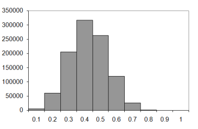
Figure 2 documents the impact of this change on the calculated value of the expected number of knots.
|
|||||||||||||||
| Figure 2 |
As you can see, it's a much better approximation. The question remains as to how well it fits for lengthy walks. Exhaustively enumerating long walks is out of the question, so we're going to have to take random samples.
We'll need an equivalent to std::random_shuffle with which we can generate them. Ideally, it should be as general as our next_state function. The trouble is that it's a bit tricky to come up with a satisfying method to randomly generate one of a fixed number of arbitrary states. The best I can think of is to use a sequential container of states and randomly generate indices into it. Admittedly, it's not very natural for integer types, but at least we can use it with any type we want. (Listing 8: Generating random states.)
    double
    rnd(double x)
    {
      return x * double(rand())/
        (double(RAND_MAX)+1.0);
    }

    template<class BidIt, class States>
    void
    random_state(BidIt first, BidIt last,
       const States &states)
    {
      while(first!=last)
      {
        *first++ = states[size_t(
           rnd(double(states.size())))];
      }
    }
|
Listing 8 |
Listing 9 illustrates the code to take a random sample of a walk of length n .
    namespace knots
    {
      void sample_crossings(
       knot_histogram &h, size_t samples);
    }

    void
    knots::sample_crossings(knot_histogram &h,
                            size_t samples)
    {
      if(h.walk_length())
      {
        std::vector<size_t> states(9);
        for(size_t i=0;i!=states.size();++i)
           states[i] = i;

        walk w(h.walk_length());

        while(samples--)
        {
          random_state(w.begin(), w.end(), states);
          h.add(crossings(w));
        }
      }
    }
|
Listing 9 |
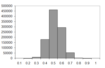
So how does the new formula rate for long walks? Figure 3 shows the results for one million samples from walks of various lengths.
|
|||||||||||||||
| Figure 3 |
Clearly, the assumption of independence is inappropriate; the calculated number of knots diverges from the observed number pretty quickly. Unfortunately, this does not bode well for the distribution I had suspected.
That distribution is the Poisson distribution. This is the distribution of the expected number of occurrences of events with exponentially distributed waiting times. Now this may not sound as general as the normal distribution since that's the limit distribution of sums of independent random numbers drawn from almost any given distribution. It would be a mistake to dismiss it too quickly though.
If the average time we need to wait before an event occurs is independent of the amount of time we have already been waiting, then the waiting times must be exponentially distributed. And these kinds of events show up a lot; consider how long we should wait before rolling a six on a fair die. Of course this is a discrete, rather than continuous, time example but should give you an idea of how common these types of events really are.
The Poisson distribution gives the probability that r events will occur given that the expected number occurrences is λ and is defined by the formula
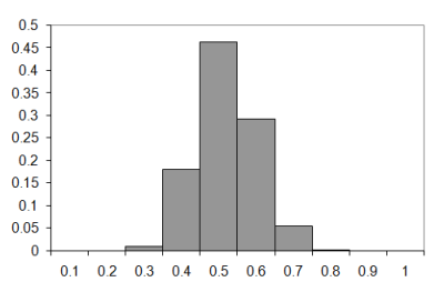
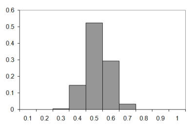
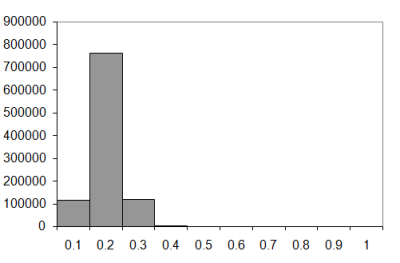
So how does it compare to the observed results? Figure 4 compares the observed and approximate histograms for a walk of nine steps.
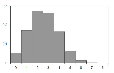
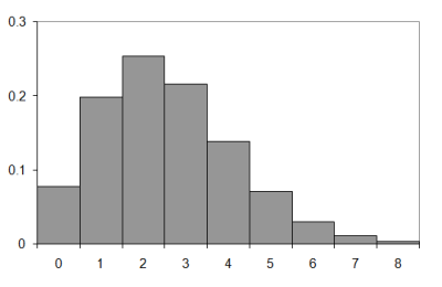
|
| Figure 4 |
Well, they're sort of similar I suppose. Not very much so, though. It seems that I was right to be concerned about the inaccuracy of the independence assumption.
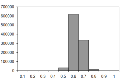
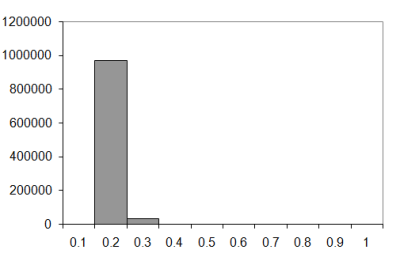
Does the situation improve for these longer walks? I suspect not given that the approximation of the expected number of knots seems to get less accurate for longer walks. Still, it's a simple matter to check, so let's take a look at some longer walks.
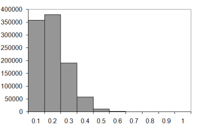
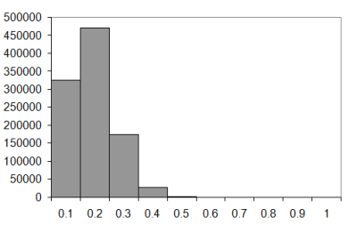
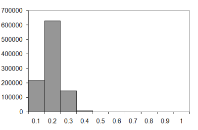
The sample distributions from which we derived the expected number of knots above are shown in Figure 5. Top left shows walks of 10 steps; top right of 20 steps; bottom left of 50 steps and bottom right of 100 steps.

|
| Figure 5 |
Figure 6 compares the difference between the observed and Poisson approximation for the one hundred step walk.
|
| Figure 6 |
As expected, the approximation is not really any better for lengthy walks.
So, we shall have to rely upon the sample data. They certainly seem to indicate that this universe favours a high proportion of self crossings and hence, presumably, knots. The question that remains is whether or not the universe is out to get us. Would we be liberated from the foul machinations of stringy things if we lived somewhere else?
Well, to answer that let's take a look at what life might be like if we lived in a universe with four spatial dimensions. Firstly, we'll need to change the position class to represent a point in three dimensional space (Listing 10).
    namespace knots
    {
      class position
      {
      public:
        position();
        position(long x, long y, long z);
        position move(long dx,long dy,long dz) const;
        bool   operator<(const position &rhs) const;
        bool   operator==(const position &rhs) const;

      private:
        long x_;
        long y_;
        long z_;
      };
    }
|
Listing 10 |
The changes to the member functions are fairly obvious, as Listing 11 illustrates.
    knots::position
    knots::position::move(long dx,
                          long dy, long dz) const
    {
      return position(x_+dx, y_+dy, z_+dz);
    }

    bool
    knots::operator<(const position &rhs) const
    {
      return x_<rhs.x_ ||
            (x_==rhs.x_ && y_<rhs.y_) ||
            (x_==rhs.x_ && y_==rhs.y_ && z_<rhs.z_);
    }
|
Listing 11 |
Next we need to update the calculation of the number of crossings in a given walk. Again, it's reasonably straightforward (Listing 12).
    size_t
    knots::crossings(const walk &w)
    {
      size_t knots = 0;
      position p(0, 0, 0);
      std::set<position> visited;

      walk::const_iterator first = w.begin();
      walk::const_iterator last  = w.end();

      visited.insert(p);

      while(first!=last)
      {
        if(*first>26) throw std::invalid_argument("");

        long dx = long(*first)%3     - 1;
        long dy = (long(*first)/3)%3 - 1;
        long dz = long(*first)/9     - 1;

        p = p.move(dx, dy, dz);
        if(!visited.insert(p).second) ++knots;
        ++first;
      }

      return knots;
    }
|
Listing 12 |
The main point here is that we now have twenty seven valid states rather than nine. The extraction of the steps in each direction follows the approach used for the two dimensional case, with a little additional complexity to cope with the third dimension.
The one million sample histograms for walks of ten, twenty, fifty and one hundred steps are illustrated in Figure 7 (knot histograms for three dimensional walks of length 10, 20, 50 and 100).
|
| Figure 7 |
The difference between the two and three dimensional walks is fairly dramatic, I'm sure you'll agree. In the two dimensional case the most probable number of knots seems to increase as a proportion of the number of steps as the walk lengthens. In the three dimensional case it seems to tend to 0.1 to 0.2 times the length of the walk.
Does this trend continue? Let's compare the results for a really long walk, say one thousand steps.
|
| Figure 8 |
I think the evidence speaks for itself; the universe really is out to get us, since it seems to have left our four dimensional neighbours relatively unmolested.
Spared from the burden of ever having to untangle the power cables for their diabolical death rays, any invading horde from the fourth dimension is well set to spring a surprise attack upon us at a moment's notice. We can only be thankful that they haven't yet done so.
I honestly believe that we are not adequately prepared for such a contingency.
Given the enormous difficulty they'll surely have tying their shoelaces, I suspect that a great many of their dread number will have to attack barefoot. I therefore suggest that we should petition the government to arm every household with an ample supply of brass tacks. If we are sufficiently alert, we should be able to stop them dead in their tracks.
In the meantime, we should continue our research. I am out of ideas, but if you, dear reader, can discover anything further please write in. The future of humanity may depend upon it.
Acknowledgements
With thanks to Andrey Biryuk and Chris Morris for proof reading this article.
References & Further Reading
Bachelier, L., Théorie de la Spéculation , PhD thesis, 1900.
Brown, R., 'A brief account of microscopical observations made in the months of June, July and August, 1827, on the particles contained in the pollen of plants; and on the general existence of active molecules in organic and inorganic bodies.' Edinburgh New Philosophical Journal , July-September, pp. 358-371, 1828.
Feller, W., An Introduction to Probability Theory and its Applications , vol. 1, 3rd ed., Wiley, 1968.
Hayes, B., 'Square Knots', American Scientist , vol. 85, num. 6, pp. 506-510, 1997
Hull, J., Options, Futures and Other Derivatives , 6th ed., Prentice Hall, 2005.
Jerome, J. K., Three Men in a Boat , J. W. Arrowsmith, 1889.
Nechaev, S., Statistics of Knots and Entangled Random Walks , arXiv:cond-mat/9812205 v1, www.arxiv.org, 1998.
Press et al., Numerical Recipes in C , 2nd ed., Cambridge, 1992.
Robbins, H., 'A Remark of Stirling's Formula', American Mathematical Monthly , vol. 62, pp. 26-29, 1955.
Theile, T. N., Om Anvendelse af mindste Kvadraters Methode i nogle Tilfælde, hvor en Komplikation af visse Slags uensartede tilfældige Fejlkilder giver Fejlene en 'systematisk' Karakter, Vidensk. Selsk. Skr. 5. Rk., naturvid. og mat. Afd., vol. 12, pp. 381-408, 1880.