Stuart Golodetz continues his survey of algorithms for segmenting images into regions.
In my last article [ Golodetz ], I described a way of segmenting images using the watershed transform and commented that the biggest problem with the results was one of oversegmentation: the image gets divided into too many regions because a region is generated for every regional minimum in the image, regardless of whether it's of any interest to us. The waterfall algorithm [ Marcotegui ], the subject of this article, is a hierarchical approach which attempts to solve this problem. (Readers may wish to consult the original paper for a more detailed justification of some of the methods involved.).
Gaussian blurring
Before we start looking at the algorithm in detail, though, it's worth observing that there are useful pre-processing steps we can take to reduce the initial number of regional minima before even applying the watershed transform. In particular, it's well worth our time to apply a Gaussian blur to the original image before taking its gradient. (There are other useful things we should do here as well, but this is an area I'm still looking into.)
Gaussian blurring is essentially a form of weighted pixel averaging based on a discrete approximation to the 2D version of the normal distribution. Many of you will doubtless be familiar with the 1D Gaussian from statistics:
              1       -x²
    gσ(x) = ———— exp( ——— )
            σ√2π      2σ²
Its 2D version can be obtained by multiplying a 1D Gaussian in the x direction with one in the y direction:
                             1       -(x²+y²)
    Gσ(x,y) = gσ(x)×gσ(y) = ———— exp( ———————— )
                            2πσ²        2σ²
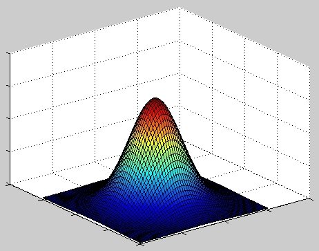
In 1D, its graph is the familiar bell-shaped curve; in 2D, we get a bell-shaped surface (see Figure 1).
|
| Figure 1 |
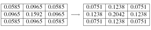
To use this for image blurring, we form a symmetric mask (see Figure 2) from the values of G σ (x,y) at discrete points in a grid centred at the origin (e.g. for a 3x3 mask, we calculate values at (-1,-1), (0,-1), (1,-1), ..., (0,0), ..., (1,1)). We then normalize the mask by dividing by the sum of all the values in it (this is done to ensure that regions of uniform intensity in the image will be unaffected by smoothing). This procedure can be used to generate masks of other sizes as well.
As an example (Figure 2), we'll calculate a 3x3 mask for the 2D Gaussian G 1 (x,y) (i.e. the Gaussian with standard deviation σ = 1). First we calculate the values of G 1 (x,y) at the grid points (i.e. we calculate G 1 (-1,-1), ...,G 1 (1,1) to give us the unnormalized mask (left); then, we normalize it by dividing through by the sum of all the values in the mask to give the final result (right).
|
| Figure 2 |
The actual blurring is done by what is known as convolving the image with the mask. This basically means overlaying the mask on each pixel of the image in turn, multiplying the value of each pixel in the mask by the value of the pixel beneath it, summing the results and using the value thus obtained as the value of the centre pixel in the blurred image. For the 3x3 mask with σ = 1, this means that if I(x,y) is the source image, M(x,y) is the mask and I'(x,y) is the blurred image, then:
| I'( x , y ) = | 0.0751 x (I( x -1, y -1) + I( x +1, y -1) + I( x -1, y +1) + I( x +1, y +1)) + |
| 0.1238 x (I( x , y -1) + I( x , y +1) + I( x -1, y ) + I( x +1, y )) + | |
| 0.2042 x I( x , y ) |
Introducing the Waterfall
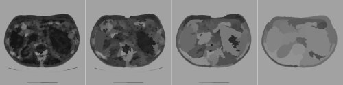
Having talked about pre-processing, we can now turn our attentions to the actual waterfall algorithm. The basic idea is to take the result of the watershed transform on the gradient of the original image and use it to produce a sequence of images by merging some adjacent regions (see Figure 3). The waterfall algorithm produces a hierarchical sequence of segmentations, starting from the original watershed result (far left). The final image will eventually be a single region (not shown).
|
| Figure 3 |
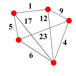
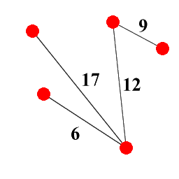
The algorithm described in [ Marcotegui ] works on the region adjacency graph (RAG) of the watershed result. This is a graph with one vertex for each region in the watershed, and weighted edges joining adjacent regions (see Figure 4). As we will see, the weights on the edges essentially determine the order of region merging, and we have a number of different options when calculating them. For now, we'll assume that we already have a suitably weighted graph, and focus on how to use it to iterate from one stage in the waterfall sequence to the next.

|
| Figure 4 |
Figure 4 shows a set of regions (left) and their region adjacency graph (right) - note that edges to the surrounding region are not shown to make things clearer.
The basic idea of a waterfall iteration involves doing something very like a watershed algorithm on the RAG. First of all, we have to find the regional minima of the graph, which in this case means its regional minimum edges (we'll define what we mean by this shortly). We then mark each such edge with a different label and carefully propagate the labels to the rest of the edges of the graph (this is an implementation of the watershed-from-markers algorithm, where the regional minimum edges are the markers). This induces a new labelling of the various regions, resulting in some of the adjacent regions being merged.
In practice, we don't run the algorithm on the RAG itself; for reasons that are fully explained in the referenced paper, the minimum spanning tree (MST) of the graph contains sufficient information that we can simply run the algorithm on that, with a corresponding gain in efficiency. To briefly recap for those who are unfamiliar with MSTs, they can be defined as follows.
Given a graph G = ( V , E , w ) with vertex set V , edge set E and weight function w : E → Z + , the set of spanning trees ST ( G ) of G is the set of subgraphs of G which are both trees (i.e. they're acyclic) and which span G (i.e. they contain every vertex in V ): see Figure 5 for an example, which shows a graph and one possible spanning tree for it.
|
| Figure 5 |
A minimum spanning tree is then simply one with a minimum total cost, i.e. a spanning tree T = ( V , E' , w )∈ ST(G) such that
  ∀(V,E″,w) ∈ ST(G)º ∑  w(e′) ≤ ∑  w(e″)
                     e′∈E′      e″∈E″
Constructing a minimum spanning tree can be done straightforwardly using Kruskal's algorithm. This involves sorting the edges in the graph into ascending order by weight, then adding the edges in ascending order to the minimum spanning tree provided they wouldn't create a cycle and invalidate the tree.
Data structures
To implement the waterfall efficiently, we're going to have to learn a bit about data structures. One of the key things we need to know about is Tarjan's data structure for disjoint set forests (I mentioned this briefly last time). This structure, designed for maintaining a collection of (mutually) disjoint sets that change over time, is widely useful and not merely restricted to our current purposes. Indeed it's the sort of thing that crops up in Computer Science degree courses [ Worrell ]! In the previous article and this one alone, this structure gets used during the fletching stage of the watershed algorithm and as part of Kruskal's algorithm, and that's before we've even mentioned its usage in maintaining the regions for the actual waterfall algorithm itself.
The idea, then, is to represent each disjoint set as a rooted tree. Finding which set an element is in is as simple as walking up the tree to the root. Unioning two sets involves finding the roots of two separate trees, and making one tree root a child of the other. For efficiency reasons, it makes sense to keep the paths to the roots of the trees as small as possible. Two tricks used to accomplish this are union-by-rank and path compression . Without dwelling on the details, the first of these tries to ensure that we're making the root of the smaller tree a child of that of the larger one, and the second changes all the parent pointers on a path to the root to point directly to the root when a 'find root' call is made: this ensures that subsequent calls on any element on the path will be constant time. The code to implement all this is shown in Listing 1, which shows Tarjan's Disjoint Set Forest.
    MAKE-SET(x)
        parent[x] ? x
        rank[x] ? 0

    FIND-SET(x)
        if x ? parent[x] then
            parent[x] ? FIND-SET(parent[x])
        return parent[x]

    LINK(x,y)
        if rank[x] > rank[y] then
            parent[y] ? x
        else
            parent[x] ? y
            if rank[x] = rank[y] then
                rank[y] = rank[y] + 1

    UNION(x,y)
        LINK(FIND-SET(x), FIND-SET(y))
|
| Listing 1 |
In the waterfall algorithm, we use such a disjoint set forest to store which regions are connected to each other. Initially, we have a tree for each region in the watershed result; as we merge regions (see Edge Elision below), we then union their respective trees. This makes region merging a very fast process, since we don't have to update the region indices for all the individual pixels in the regions. Instead, each pixel maintains the label it was originally given by the watershed transform: this can then be used to look up the correct region value in the disjoint set forest associated with any given level of the waterfall. The space savings are also noticeable: instead of storing a full image of labels for each waterfall iteration, we need only store the results of the watershed and a disjoint set forest for each level of the hierarchy.
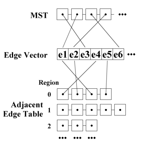
The other data structures we'll use are for maintaining edges. The layout is as shown in Figure 6. We maintain an array (in practice, a std::vector ) which stores all the edges we'll be referring to (these can either be all the edges in the RAG, or all the edges in the initial MST if we want to be particularly space-efficient). The MST is represented as a list of edge pointers sorted in ascending order of edge weight. Finally, we store an edge adjacency table, which stores lists of pointers to edges which are adjacent to each of the various regions.
|
| Figure 6 |
Figure 6 shows the data structures used for the waterfall algorithm: some of the pointers aren't shown for reasons of clarity.
Step 1: Finding the Regional Minimum Edges
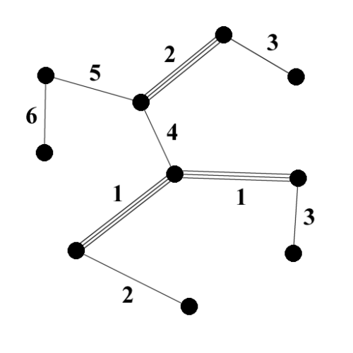
A regional minimum edge (RME) of a graph G is a connected subgraph of G whose own edges have equal weight and whose adjacent edges in G have strictly higher weights (see Figure 7).
|
| Figure 7 |
Figure 7 shows an example graph and its RMEs (drawn as triple edges). Note that the two edges with a weight of 1 are part of the same RME.
To find all the regional edges in the MST, we run through all the edges in the MST and flood outwards from each one to determine (a) whether it's part of an RME and (b) the extent of the RME if so (see Listing 2, the flooding algorithm for finding RMEs). We do this by maintaining two things: an equal edges list, which holds all the edges that may form part of the current hypothetical RME, and an adjacent edges queue, which holds all unprocessed edges which are adjacent to one of the aforementioned equal edges. We process all adjacent edges one at a time. If we see a lower edge, this isn't an RME. If we see an equal edge, we add it to the list of edges which may be in the RME and add its adjacent edges to the queue. If we see a higher edge, we ignore it. If we empty the adjacent edges queue without seeing a lower edge, we've found an RME, so we add it to the list, mark all the edges in it as being part of an existing minimum (to avoid later duplication) and continue from the top with the next MST edge.
    Vector<EdgeList> rmeArray;

    foreach(Edge startEdge   mst)
      // The edge is already part of a regional
      // minimum edge. If we processed it, we'd
      // end up duplicating that minimum edge,
      // so skip over it.
      if(startEdge->minimum) continue;

      // Maintain a list of equally-valued edges
      // which may form part of the same RME.
      EdgeList equalEdges;
      EdgeQueue adjacentEdges;

      // Maintain a queue of pending edges so they
      // can be unmarked again later.
      EdgeQueue pendingEdges;

      // Mark the initial edge to ensure it isn't
      // wrongly identified as being adjacent to
      // itself.
      startEdge->pending = true;
      pendingEdges.push(startEdge);

      add_adjacent_edges(startEdge,
                         adjacentEdges,
                         pendingEdges);

      bool isMinimum = true;
      while(!adjacentEdges.empty())
        Edge adjacent = adjacentEdges.pop();
        if(adjacent->value < startEdge->value)
          // If its value is less than the start
          // edge, then the start edge is not a
          // minimum.
          isMinimum = false;
          break;
        elseif(adjacent->value == startEdge->value)
          equalEdges.push_back(adjacent);
          add_adjacent_edges(adjacent,
                             adjacentEdges,
                             pendingEdges);

      // Unmark all the pending edges.
      while(!pendingEdges.empty())
        Edge e = pendingEdges.pop();
        e->pending = false;

      if(isMinimum)
        // Add the start edge to the list now that
        // we know we've found a minimum.
        equalEdges.push_front(startEdge);
        for(Edge e   equalEdges)
          e->minimum = true;
        rmeArray.push_back(equalEdges);
|
| Listing 2 |
Edge elision
In my implementation of the waterfall, no actual relabelling of the regions is done. Instead, the same effect is achieved by merging regions via the mechanism of eliding (i.e. removing) edges in the RAG. The process of edge elision is slightly intricate because all the relevant data structures need to be updated. We need to union the disjoint set forest trees associated with the regions at either end of the edge, we need to splice the edge adjacency lists together (thus adding the list of all the edges adjacent to one of the regions to that of the other) and we need to do various bits of additional housekeeping (see Listing 3, edge elision). One important step is to mark the edge as elided, so that it can be removed from the MST in Step 4 of the algorithm (see below).
    ELIDE-EDGE(e)

    unsigned int u = e->u;
    unsigned int v = e->v;

    unsigned int setU = forest.find_set(u);
    unsigned int setV = forest.find_set(v);

    forest.union_nodes(u, v);

    // Mark the edge as elided for when we come to
    // later rebuild the MST.
    e->value = -1;

    // forest.find_set(u) == forest.find_set(v)
    unsigned int parent = forest.find_set(u);

    // Add all the edges adjacent to the child
    // regions to the parent region in the
    // adjacency table.
    EdgeList parentList = adjacencyTable[parent];
    if(setU != parent)
      parentList.splice(parentList.end(),
                        adjacencyTable[setU]);
    if(setV != parent)
      parentList.splice(parentList.end(),
                        adjacencyTable[setV]);

    // Remove the elided edge from the parent list.
    parentList.remove(e);

    // Update the region values.
    Value parentValue = forest.value_of(parent);
    Value uValue = forest.value_of(setU);
    Value vValue = forest.value_of(setV);
    if(uValue > parentValue) parentValue = uValue;
    if(vValue > parentValue) parentValue = vValue;
|
| Listing 3 |
Step 2: Eliding the RMEs
Having found the RMEs in Step 1 (above), the next part of the actual algorithm is to elide them. This is done as an alternative to assigning them all the same label (as per the original waterfall description).
Step 3: Marker propagation
Once we've 'labelled' the marker regions by eliding all the RMEs connecting them, the next step is to propagate the markers to the rest of the MST using a flooding process, at each stage processing an adjacent edge with lowest cost. The ideal data structure for this is a priority queue. The algorithm (see Listing 4, marker propagation) works as follows: we initialise the queue with any edges which are adjacent to RMEs and mark the regions joined by the RMEs as already processed. We then repeatedly pop the lowest cost edge from the queue, merging the regions it connects if one of them is unmarked, and ignoring it otherwise. If an edge is elided, its own adjacent edges are also added to the queue.
    // Flags indicating whether a region has been
    // marked or not.
    Vector<char> markedRegion(forest.node_count());

    PriorityQueue<Edge> pq;
    EdgeQueue pendingEdges;

    // Add all the edges adjacent to RMEs to the
    // priority queue.
    foreach(EdgeList rme   rmeArray)
      foreach(Edge e   rme)
        add_adjacent_edges(e, pq, pendingEdges);
        int setU = forest.find_set(e->u);
        int setV = forest.find_set(e->v);
        markedRegion[setU] = 1;
        markedRegion[setV] = 1;

    // Process each edge in ascending order of
    // value, adding adjacent edges to the priority
    // queue each time.
    while(!pq.empty())
      Edge e = pq.pop();

      int setU = forest.find_set(e->u);
      int setV = forest.find_set(e->v);

      // If this region connects a marked region to
      // an unmarked one, it needs processing.
      // Otherwise it should be ignored. Note that
      // because of the way the propagation works,
      // any edge will either connect a marked
      // region to an unmarked one, or it will
      // connect two marked regions.
      if(!markedRegion[setU] || !markedRegion[setV])
        ELIDE-EDGE(e);
        markedRegion[setU] = 1;
        markedRegion[setV] = 1;
        add_adjacent_edges(e, pq, pendingEdges);

    // Unmark all the pending edges.
    while(!pendingEdges.empty())
      Edge e = pendingEdges.pop();
      e->pending = false;
|
| Listing 4 |
Step 4: Rebuilding the MST
The final step of the algorithm is to rebuild the MST so that it's ready for the next waterfall iteration. This turns out to be an almost trivial process, since we just have to remove any elided edges from the tree. Since we carefully marked them all with a value of -1 when they were elided, all we have to do is run through the list representing the MST and remove any edges whose value is -1 (in C++, this can be handled extremely simply using a remove_if call).
Edge valuations
One issue we haven't yet touched on is how to generate suitable weights for the edges of the region adjacency graph. Since these weights determine the order of region merging, they have a substantial effect on the output of the whole algorithm, so it's important to choose them carefully.
There are a number of different options available. The simplest approach, known as lowest pass, valuates each edge with the height of the lowest pass point on the border between the regions it joins. One advantage of this method is that it's easy to calculate: you just run through all the pixels in the watershed result, find any border pixels (pixels which have at least one neighbour with a different label) and update the lowest pass between any two regions as necessary.
Lowest pass isn't always the best method to use, however, and several other sensible valuations have been proposed. These generally focus on the idea of dynamics, which involves thinking about either the height (contrast dynamics), the surface area (area dynamics) or the volume (volume dynamics) of the water in the catchment basins of the adjacent regions at the point when they would meet during the flooding process (i.e. the point where a watershed is built to keep them apart). These all produce different results and some experimentation is needed to see which may be the most appropriate in a given situation. Another interesting valuation can be found in [ Climent ], where the authors use some knowledge about the human perception of shapes to define a dynamic which (on their test images at any rate) produces more visually-pleasing results than (in particular) the volume dynamic, with which they contrast it.
My own work is currently using lowest pass, but I plan to experiment further with the other valuations in due course.
Conclusion
From my own experiments with the waterfall algorithm, I can attest to the fact that the results of waterfall segmentation seem to be much more useful than the original watershed result. It's not that any particular image in the waterfall sequence gives us the ideal segmentation: that would be far too easy. What the waterfall does give us is a lot of connected regions (in the various different images in the sequence) to work with further. With these results, we can go on to use region analysis and classification strategies to identify which regions in the various waterfall iterations correspond to features of interest in our original image. Waterfall thus takes us one step closer to our original goal of automatic segmentation. How to do the actual region analysis and classification is still a research problem, but one I hope to continue working on in the near future.
Till next time...
References
[ Climent] 'Visually Significant Dynamics for Watershed Segmentation', Joan Climent and Alberto Sanfeliu. In Proceedings of the 18th International Conference on Pattern Recognition (ICPR '06), 2006.
[ Golodetz] 'Watersheds and Waterfalls (Part 1)', Stuart Golodetz, Overload 83 , February 2008.
[ Marcotegui] 'Fast Implementation of Waterfall Based on Graphs', Beatriz Marcotegui and Serge Beucher. In Mathematical Morphology: 40 Years On , Springer Netherlands, 2005.
[ Worrell] 'Data Structures for Disjoint Sets', James Worrell. Advanced Data Structures and Algorithms course notes, Oxford University, 2006.